COURSE DESCRIPTION

请用英语在微信群里面提问. 所有的课程文件都在学校云盘里面，只有在交作业的时候会用网络学堂. 每节课后会发 html 格式的 note.

7 modules：

• Light

• Matter under astrophysical conditions

  (Extreme conditions)

• Evolution

• Atmospheres

• Birth

  How do stars and planets form

• Exo-planets

• Planet Dynamics

参考书目：

• Main: B. O. B. (Big Orange Book —— Modern Astrophysics)
• Stellar Structure and Evolution
• Astrophysics of Planet Formation
• Dynamics of Planetary Systems
• Solar System Dynamics

html note 是 reveal.js 写的，在老师的主页上. 另外是 Princeton 的天文学讲义，很多课堂问题会来自里面.

分数组成有五个方面：考试、Quiz、Problem Set、Presentation 和 report 里面取一个最高值、前三项里面取一个最高值，都是 20%20\% 分数. 其中 report 是 optional，如果写了就可以代替后两项的分数.

Problem Set：

一共六次，一般是一个单元一次.

不能抄，可以用 AI，但是不能完全没有自己的想法，"use your own words"，当老师提问时你应该能够自己回答出来.

可以交 .pdf 也可以手写，如果是一个格式很棒的 .pdf 会有一定加分.

迟交扣分.

提示

如果要画图，请优化你的图片，不要上交一些没有标题、scale 奇怪的东西；另外，公式使用标准的格式，不需要写出很具体的数值计算过程.

课程上会使用 Gaussian Unit System，作业中可以用 SI，但是请 be consistent.

量纲分析：用来检查方程，或者做简单估计.

如果一个质量为 MM、半径 RR 的均匀球状气体在真空中坍缩，求时间.

量纲分析表明：

t=O(R3GM)t = O\left(\sqrt{\frac{R^3}{GM}}\right)

---

估计一头牛的重量. 线度大约是 1 m1\text{ m}，密度和水差不多，所以是 1 t1\text{ t} 重左右.

助教会在课外时间办一次 matplotlib 的讲座，大家自愿去听.

Research Project：

今年的主题关于 MESA. 可以自行选择列表中的 project 主题. 最后两周每一个人都要做自己的 presentation.

Module 1 LIGHT

首先，我们知道光是一种电磁现象. 整个电磁波谱非常广，从微波到可见光再到 gamma 射线. 天文上比较重要的谱线是 21 cm21\text{ cm} 线，由 He 的某一个自旋翻转造成.

Quantum Blocks：所谓的相空间量子化. 我们可以在相空间中的小格子里面放 FF 个粒子，如果粒子是 fermion，那么每一个格子只能放 0 或者 1 个粒子，考虑自旋能够多放一个；如果是 boson，那么一个格子可以放任意多个粒子. 一个格子的体积是

d3xd3p=h3\text{d}^3x\text{d}^3p = h^3

现在我们算总的粒子数，应该是

n photons=∫Fh3⋅d3xd3pn\text{ photons} = \int\frac{F}{h^3}\cdot\text{d}^3x\text{d}^3p

不对空间积分，我们会得到粒子的空间数密度，

nph=∫Fh3⋅d3p=4πh3∫Fp2dpn_{\text{ph}} = \int\frac{F}{h^3}\cdot\text{d}^3p = \frac{4\pi}{h^3}\int Fp^2\text{d}p

现在需要能动关系. 我们知道对于光子，

E=hν,p=hνc⟹nph=4πc3∫Fν2dνE =h\nu,\quad p = \frac{h\nu}{c}\Longrightarrow n_{\text{ph}} = \frac{4\pi}{c^3}\int F\nu^2\text{d}\nu

现在要知道 F=F(ν)F = F(\nu) 是一个什么样的东西. 根据 Boltzmann 统计，光子随着 ν\nu 的分布应该正比于一个因子，这写成：

P(1)∝e−hν/kBT=e−x,P(2)∝P2(1)=e−2x,x=hνkBTP(1)\propto e^{-h\nu/k_BT} = e^{-x},\quad P(2) \propto P^2(1) = e^{-2x},\quad x = \frac{h\nu}{k_BT}

对这个数列求和 (相当于做归一化)，获得光子分布函数 (也就是 Bose - Einstein 分布)：

nˉ=∑i=0∞ne−nx∑i=0∞e−nx=1ex−1\bar{n} = \frac{\displaystyle{\sum_{i=0}^\infty ne^{-nx}}}{\displaystyle{\sum_{i=0}^\infty e^{-nx}}} = \frac{1}{e^x-1}

F=π⋅nˉF = \pi\cdot\bar{n}，因为是球面积分过一次的结果. 于是光子空间数密度的谱是

dnphdν=4πc3⋅ν2⋅πex−1\frac{\text{d}n_{\text{ph}}}{\text{d}\nu} = \frac{4\pi}{c^3}\cdot\nu^2\cdot\frac{\pi}{e^x-1}

能量密度谱为

uν=hν⋅dnphdν=8πhν3c3⋅1ehν/kBT−1u_\nu = h\nu\cdot\frac{\text{d}n_{\text{ph}}}{\text{d}\nu} = \frac{8\pi h\nu^3}{c^3}\cdot\frac{1}{\displaystyle{e^{h\nu/k_BT}-1}}

总的能量密度是这个密度谱对 ν\nu 的积分，

Utot=∫uνdν=4σsbcT4,σsb=2π5kB415h3c2(Stefan - Boltzmann constant)U_{\text{tot}} = \int u_\nu \text{d}\nu = \frac{4\sigma_{\text{sb}}}{c}T^4,\quad \sigma_{\text{sb}} = \frac{2\pi^5k_B^4}{15h^3c^2}\quad(\text{Stefan - Boltzmann constant})

当然我们知道这个积分并不容易... 大家有兴趣可以下课尝试.

上面算得的 uνu_\nu 是一个单位体积内，ν∼ν+dν\nu\sim\nu+\text{d}\nu 之间的光所携带的能量. 现在考虑从这个方块体积的某一个面 (面积 dA\text{d}A) 有光子逃逸出来，在一个短时间 dt\text{d}t 内、朝着 dΩ\text{d}\Omega 空间角方向. 这样的一个分布可以写成

dEdAdtdΩ=12uνc2π=uνc4πcos⁡θ\frac{\text{d}E}{\text{d}A\text{d}t\text{d}\Omega} = \frac{\displaystyle{\frac{1}{2}u_\nu c}}{2\pi} = \frac{u_\nu c}{4\pi}\cos\theta

其中，分子上的 1/21/2 来源于只有一半光子向外，另一半是向内的；分母上的 2π2\pi 来源于 4π4\pi 立体角内部只有一半是往体积的外部的.

(如果只看法向的话) 这就是黑体辐射的光功率谱，我们称之为 Planck 公式，

Iν=Bν(T)=2hν3c2⋅1ehν/kBT−1I_\nu = B_\nu(T) = \frac{2h\nu^3}{c^2}\cdot\frac{1}{e^{h\nu/k_BT}-1}

下一步对半个立体角和全频率积分，

dEdAdt=∫dν∫0π/2∫02π2hν3c2⋅1ehν/kBT−1⋅cos⁡θsin⁡θdθdϕ=c4π∫uνdν‾Bν(T)⋅2π(sin⁡2θ2)0π/2=c4π⋅Utot⋅2π⋅12=σsbT4\begin{aligned} \frac{\text{d}E}{\text{d}A\text{d}t} &= \int\text{d}\nu\int_0^{\pi/2}\int_0^{2\pi}\frac{2h\nu^3}{c^2}\cdot\frac{1}{e^{h\nu/k_BT}-1}\cdot\cos\theta\sin\theta\text{d}\theta\text{d}\phi\\\\ &= \frac{c}{4\pi}\underset{B_\nu(T)}{\underline{\int u_\nu\text{d}\nu}}\cdot2\pi\left(\frac{\sin^2\theta}{2}\right)^{\pi/2}_0\\\\ &= \frac{c}{4\pi}\cdot U_{\text{tot}}\cdot2\pi\cdot\frac{1}{2} = \boxed{\sigma_{\text{sb}}T^4} \end{aligned}

这是 Stefan - Boltzmann 定律，对一个球面而言总辐射功率为 L=4πR2⋅σsbT4L = 4\pi R^2\cdot\sigma_{\text{sb}}T^4.

如果我们观察太阳的辐射功率谱曲线，会发现曲线和标准的黑体辐射曲线并不完全重合，这是因为太阳并不是一个标准的黑体.

Bν(T)B_\nu(T) 对 ν\nu 求导，得到 Wien 公式，

λmax⁡=0.2898 cm⋅KT\lambda_{\max} = \frac{0.2898\text{ cm}\cdot\text{K}}{T}

长波下，应该变成 Rayleigh - Jeans 公式，

Bν(T)=2ν2kBTc2B_\nu(T) = \frac{2\nu^2k_BT}{c^2}

但是 Bλ(T)B_\lambda(T) 并不简单地是将 ν=c/λ\nu = c/\lambda 代入，而是应该先变成 Bλ(T)B_\lambda(T) 再近似，最后的结果应该是 Bλ(T)∼λ−4B_\lambda(T)\sim\lambda^{-4}.

下面我们说一些测量方面的问题.

/Definition/ (par sec\text{par sec} 的定义)

我们在一年之中相隔半年的两个时刻观察同一颗恒星，看到它的天球坐标变化了一个角度 pp，那么就有一个简单的几何关系：

1 A.U.d=tan⁡p≈p\frac{1\text{ A.U.}}{d} = \tan p \approx p

这里的 dd 是恒星离我们的距离. 1 par sec1\text{ par sec} 定义为 p=1′′p = 1'' 对应的 dd，大约是 33 光年左右.

/Definition/ (星等的定义)

相对星等 mm (magnitude) 定义为

m=−2.5log⁡10FFrefm = -2.5\log_{10}\frac{F}{F_{\text{ref}}}

(这里的 FF 是到达地球的光通量 flux) 星等差为

m1−m2=−2.5log⁡10F1F2m_1-m_2 = -2.5\log_{10}\frac{F_1}{F_2}

---

绝对星等 MM 定义为：

m−M=−2.5log⁡10L/d2L/(10 pc)2=5log⁡10d10 pcm-M = -2.5\log_{10}\frac{L/d^2}{L/(10\text{ pc})^2} = 5\log_{10}\frac{d}{10\text{ pc}}

同时星等在不同的颜色上是不同的，可以通过不同颜色比较来判断恒星的颜色.

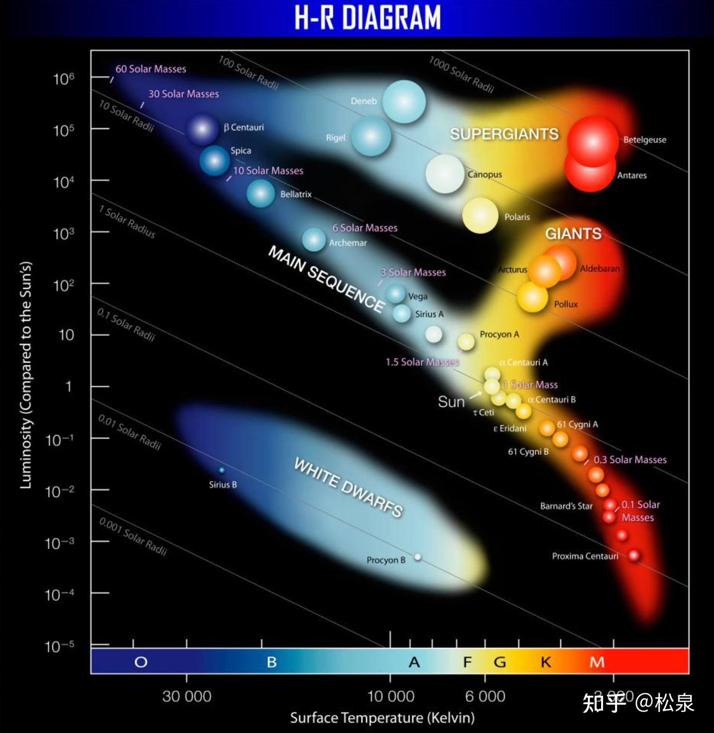
终于我们可以开始介绍 Hertzsprung-Russell diagram 图 (HR 图)，这种图以恒星绝对星等或光度为纵轴，光谱类型或色指数为横轴，用来描述恒星的光谱特性.

如图所示：