今天讲的内容是数据被截断 (truncated) 或者被模糊 (censored).

一个简单的例子是，我们望向夜空，一定有很多星星根本看不到，但是我们完全不知道哪些看到了哪些没看到，比例是多少，我们只能看到我们看到的，这就是截断；如果我们用射电望远镜或者光学望远镜观察，可能后者可以看到一个源，但是前者什么都看不到，这时候我们可以确定有什么在那里，但是不知道信号到底有多强，这就是模糊.

先看一个文章：arXiv:1502.02201. 能够看到不同的 gamma 射线源之间能够形成一个近乎完美的直线，但是其来源从太阳到宇宙的远古背景、尺度跨越极大，这真的对吗？

「Absence of evidence is not evidence of absence.」

Selection Effects and Biases

我们的数据有很多人为的成分，比如「一定要 3σ3\sigma 才是一个真的信号」，或者是望远镜没有能力看到太暗弱的星体. 但是「没有看到」这件事本身也是一个事实，也能提供信息 (比如这一块区域前景有遮挡，或者这个区域的物质密度较低)，也能被用来做统计.

没有看到的话，我们不能对这个区域的单个物体做出确认，但是我们可以对这个区域做整体的统计推断.

天文上，最常见的一种「看不到」的东西是「距离」.

/Example/ (Toy Universe)

在一个平直时空的球形宇宙中撒 10610^6 个点，均匀分布，光度按照分布函数 p(L)∝L−3p(L)\propto L^{-3} 来分配，Lmin⁡=1L_{\min}=1.

那么流量是

F=L4πD2F=\frac{L}{4\pi D^2}

探测器能够看到的是流量，要求流量 >10>10 才能被看见. 现在来做模拟，

import numpy as np
import matplotlib.pyplot as plt
 
rng = np.random.default_rng(seed=42)
N = int(1e6)
 
# Generate uniform distribution in volume
D = rng.uniform(0, 1, N)**(1/3)
 
# Generate power-law luminosities
L_min = 1
L = L_min * rng.uniform(0, 1, N)**(-0.5)
 
# Plot Hubble diagram
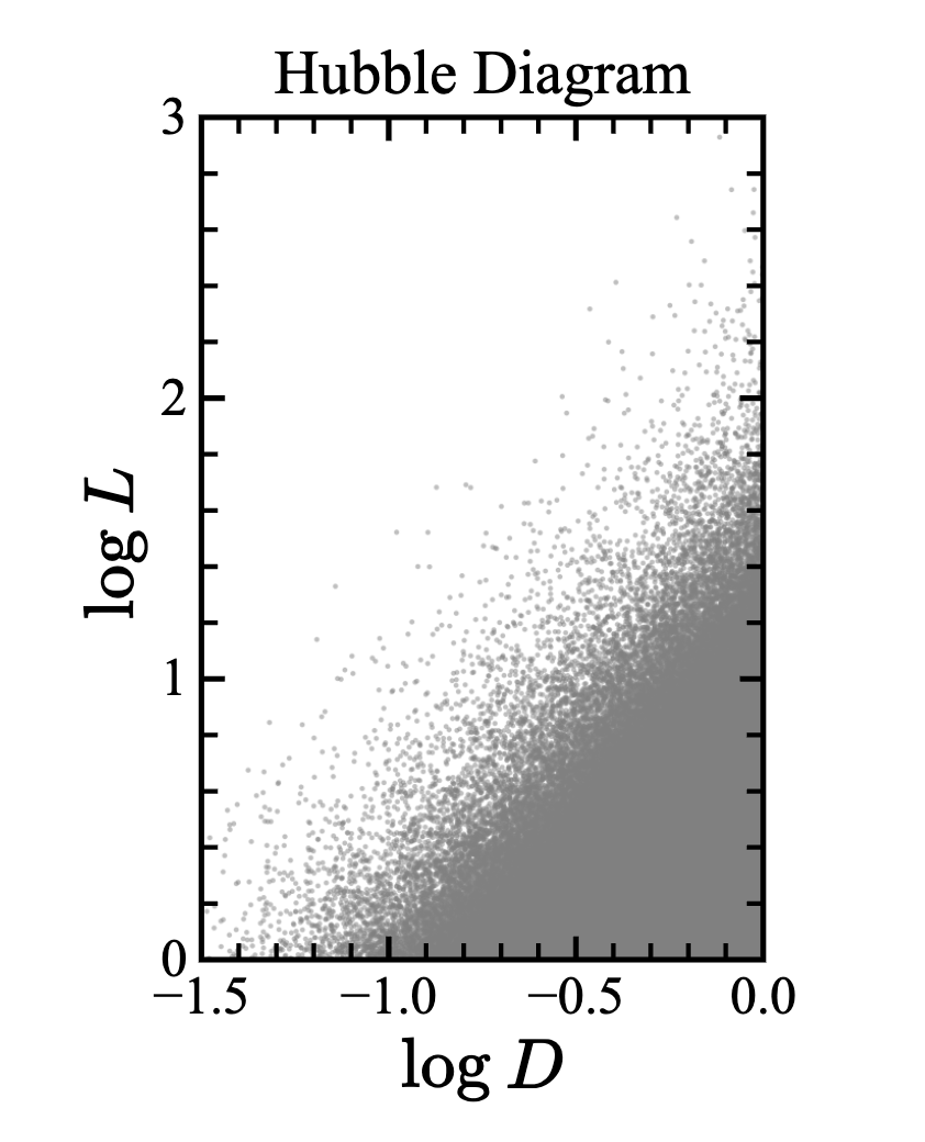
plt.scatter(np.log10(D), np.log10(L), s=0.5, c='gray', alpha=0.5)

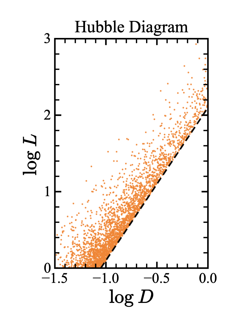
对模拟结果画 Hubble 图 (log⁡L\log L - log⁡D\log D 图)，理应是右下角的星比较多；但是如果加上观测极限，那么会在图上切割出一个 L∝D2L\propto D^2 的直线，那么我们会得到错误结果 —— 距离越远，光度越大.

这是因为，流量 FF 完全是三维时空的几何效应，那么最后得到的东西完全不会和光度分布函数有任何联系.

---

现在对两种星做测量，这两种星的光度分布函数分别为

P1(L)∝L−3,P2(L)∝L−γe−αLP_1(L)\propto L^{-3},\quad P_2(L)\propto L^{-\gamma}e^{-\alpha L}

然后我们用有探测极限的探测器去看这些星的两个波段 L1L_1 和 L2L_2，然后画 log⁡L1\log L_1 - log⁡L2\log L_2，要求最后画在图上的点必须要是两个波段都被探测到的点. 于是我们发现两种不同的星在这个图上竟然能够形成一个线性的结果.

这也说明了一开始的那篇文章为什么是错的.

这样的选择效应被称为 Malmquist 效应.

但是不仅仅是观测极限，我们还有误差：比如暗的东西可以被测为亮的东西，亮的东西可以被测为暗的东西，但是因为亮的东西比较少、暗的东西比较多，而跳变是均匀的，所以我们看到的东西里面暗的东西比真实的更多.

这是 Eddington 效应. 当我们对误差的分布很了解时，可以把这样的效应给去掉.

Population Estimation

即使有很多误差和限制，我们还是想要估计 luminosity function.

一个最笨的办法是，我们知道观测极限会在图上割掉一块，所以选出一个没有被割掉的区域，里面的样本就会是完备的样本，得到无偏的估计.

缺点是：

• 每次只能用很小的一部分数据，噪声大、数据浪费
• 每次的区域只有一部分光度函数，要靠几个区域才能叠加出一个范围足够的光度分布.

改进思路是 Vmax⁡V_{\max} 算法. 我们认为每一个被看到的源能够代表一系列的源，看到的这个源在最大距离 (由观测极限决定) 的球内任意一点都会被看到，只是碰巧在这个位置被看到了而已. 被看到了就意味着它均匀分布在整个最大距离的球内.

计算这个最大距离球的体积 Vmax⁡V_{\max}，把 1/Vmax⁡1/V_{\max} 作为这个源的权重，求和算分布函数. 这种方法相当于把更暗的星系算了更大的权重，强行拉回整个函数.

import numpy as np
 
def calc_Vmax(luminosity, flux_limit):
  """Calculate maximum accessible volume"""
  D_max = np.sqrt(luminosity / (4 * np.pi * flux_limit))
  V_max = (4/3) * np.pi * D_max**3
  return V_max
 
def luminosity_function_Vmax(luminosity, flux_limit, bin_edges):
  """Estimate luminosity function using the Vmax method"""
  Vmax = calc_Vmax(luminosity, flux_limit)
  lf, _ = np.histogram(luminosity, bins=bin_edges,
                       weights=1/Vmax)
  bin_widths = np.diff(bin_edges)
  lf /= bin_widths  # Normalize by bin widths
  return lf

但是这种算法的缺点是，依赖于「均匀」的密度，如果是 Gaussian 型的密度就没办法把函数「拉回来」.

不依赖于密度均匀的方法是 C−C^- method：画距离和绝对星等的关系图，我们能够看到的范围是 直线下方的区域.

在能看到的区域里面画一个矩形和一个矩形微元，分别有 C(Mk)C(M_k) 和 dN(Mk)\text{d}N(M_k) 个星点，这个比例可算：

df=dN(Mk)C(Mk)\text{d}f=\frac{\text{d}N(M_k)}{C(M_k)}

然后扩大这两个矩形区到不能观测的区域内，因为我们假设「距离和光度相互独立」，所以上述比例并不变化，可以重建真实的分布.

from astroML.lumfunc import binned_Cminus
 
def luminosity_function_Cminus(luminosity, distance,
      flux_limit, M_bin_edges, mu_bin_edges):
  """Estimate luminosity function using the C- method"""
  # Toy quantity conversions (constants omitted)
  mu = 5 * np.log10(distance)           # distance modulus
  M = -2.5 * np.log10(luminosity)       # absolute magnitude
  m = M + mu                            # apparent magnitude
  # Select objects above the flux limit
  m_max = -2.5 * np.log10(flux_limit)
  mask = (m <= m_max)
  M, mu = M[mask], mu[mask]
  # Truncation limits
  M_max = m_max - mu        # faintest M visible at each mu
  mu_max = m_max - M        # largest mu visible at each M
  # Estimate LF using C- method
  p_mu, p_M = binned_Cminus(mu, M, mu_max, M_max,
                    mu_bin_edges, M_bin_edges, normalize=True)
  return p_M

Survival Analysis with Censored Data

这个名字来源于医学，他们做实验的时候小白鼠可能会死，这一部分数据就缺失了，因此要想办法把数据凑回来.

还是用 Toy Universe. 但是现在我们从光学 (L1L_1) 和 X - ray 波段 (L2L_2) 来探测，分布分别是 ∝L−3\propto L^{-3} 和 ∝L−2\propto L^{-2}. 然后光学的观测极限是 Fmin⁡=10F_{\min}=10，X - ray 的观测极限是 Fmin⁡=50F_{\min} = 50.

我们只对那些光学能看到的源做 X - ray 探测. 现在数据分为两类：

• Detected：光学上看到了、射电上也看到了
• Censored：光学上看到了、射电上没看到.

把模拟结果画出来研究相关性. 假设数据 (xi,yi)≡(log⁡Lopt,i,log⁡LX,i)(x_i,y_i)\equiv(\log L_{\text{opt},i},\log L_{\text{X},i}). 然后做模型选择和参数估计. 结果得到了 8σ8\sigma 的置信度确定 yiy_i 和 xix_i 相关，这是不合理的，是假的相关性.

如果我把那些 censored 的点加进来呢？立刻将置信度压低到 0.04σ0.04\sigma、Bayes 因子的对数值到 −3.3-3.3，Occam's Razor 应该要起作用了. 这个结果非常好，给我们的启示是 —— 用上你所有的数据，我们能够还原出正确的结果.

Exercise: Toy Universe

生成一个平直时空中的球形宇宙，均匀分布 10610^6 星点. 光度分布 P(L)∝L−2P(L)\propto L^{-2}，Lmin⁡=1L_{\min}=1. 观察当观测极限是 1010 的时候的 bias，用 Vmax⁡V_{\max} 方法修正这一个 bias.

利用 Gaussian 型误差分布来构造一个 Eddington bias.