Householder matrices are square matrices of the form
$$ P = I - \beta v v^T$$
where $\beta$ is a scalar and $v$ is a vector. It has the useful property that for suitable chosen $v$ and $\beta$ it makes the product $P x$ to zero out all of the coordinates but one, that is, $P x = |x| e_1$. The following code, given $x$, finds the values of $\beta, v$ that verify that property. The algorithm can be found in several textbooks 1
def house(x):
    """
    Given a vetor x, computes vectors v with v[0] = 1
    and scalar beta such that P = I - beta v v^T
    is orthogonal and P x = ||x|| e_1

    Parameters
    ----------
    x : array, shape (n,) or (n, 1)

    Returns
    -------
    beta : scalar
    v : array, shape (n, 1)
    """
    x = np.asarray(x)
    if x.ndim == 1:
        x = x[:, np.newaxis]
    sigma = linalg.norm(x[1:, 0]) ** 2
    v = np.vstack((1, x[1:]))
    if sigma == 0:
        beta = 0
    else:
        mu = np.sqrt(x[0, 0] ** 2 + sigma)
        if x[0, 0] <= 0:
            v[0, 0] = x[0, 0] - mu
        else:
            v[0, 0] = - sigma / (x[0, 0] + mu)
        beta = 2 * (v[0, 0] ** 2) / (sigma + v[0, 0] ** 2)
        v /= v[0, 0]
    return beta, v
As promised, this computes the parameters of $P$ such that $P x = |x| e_1$, exact to 15 decimals:
>>> n = 5
>>> x = np.random.randn(n)
>>> beta, v = house(x)
>>> P = np.eye(n) - beta * np.dot(v, v.T)
>>> print np.round(P.dot(x) / linalg.norm(x), decimals=15)
[ 1. -0. -0.  0. -0.]
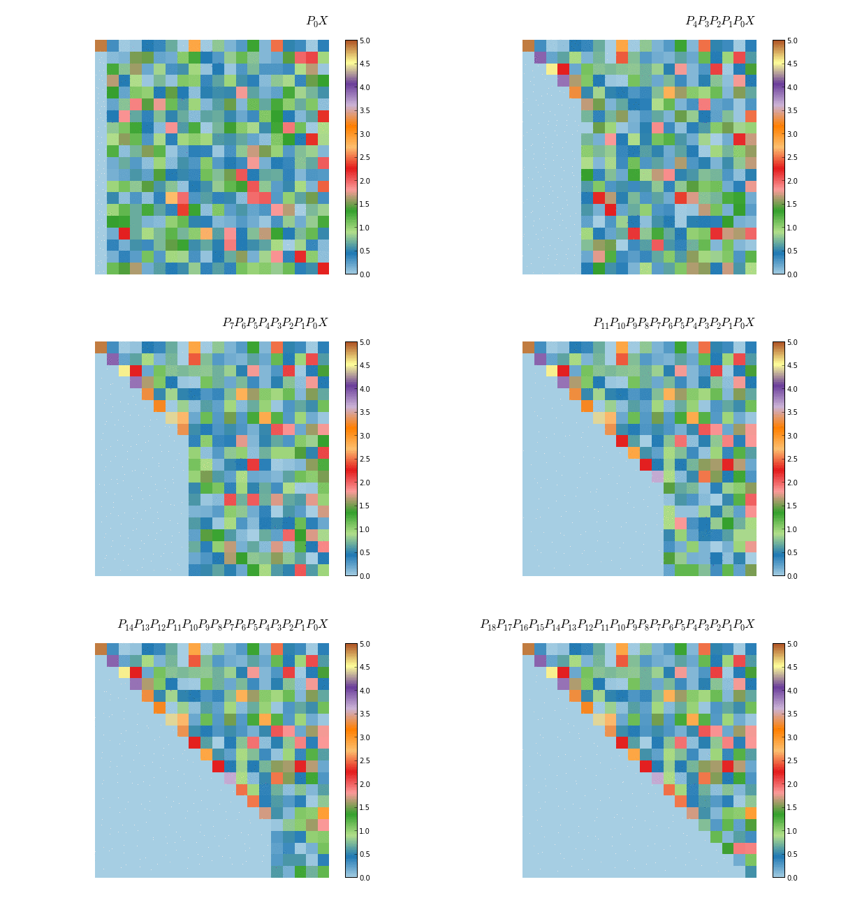
This property is what it makes Householder matrices useful in the context of numerical analysis. It can be used for example to compute the QR decomposition of a given matrix. The idea is to succesively zero out the sub-diagonal elements, thus leaving a triangular matrix at the end. In the first iteration we compute a Householder matrix $P_0$ such that $P_0 X$ has only zero below the diagonal of the first column, then compute a Householder matrix $P_1$ such that $P_1 X$ zeroes out the subdiagonal elements of the second column and so on. At the end we will have that $P_0 P_1 ... P_n X$ is an upper triangular matrix. Since all $P_i$ are orthogonal, the product $P_0 P_1 ... P_n$ is again an orthogonal matrix, namely the $Q$ matrix in the QR decomposition.
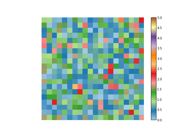
If we choose X as 20-by-20 random matrix, with colors representing different values
we can see the process of the Householder matrices being applied one by one to obtain an upper triangular matrix
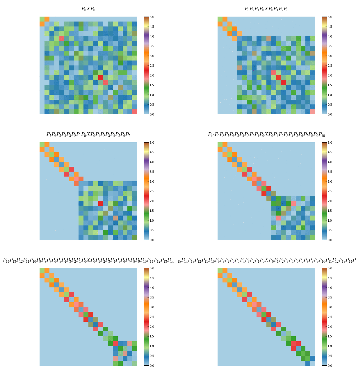
A similar application of Householder matrices is to reduce a given symmetric matrix to tridiagonal form, which proceeds in a similar way as in the QR algorithm, only that now we multiply by the matrix $X$ by the left and right with the Householder matrices. Also, in this case we seek for Householder matrices that zero out the elements of the subdiagonal plus one, instead of just subdiagonal elements. This algorithm is used for example as a preprocessing step for most dense eigensolvers