





:og_image: http://fa.bianp.net/blog/images/2014/mprof_example.png
One of the lesser known features of the memory_profiler package is its ability to plot memory consumption as a function of time. This was implemented by my friend Philippe Gervais, previously a colleague at INRIA and now at Google.
With this feature it is possible to generate very easily a plot of the memory consumption as a function of time. The result will be something like this:
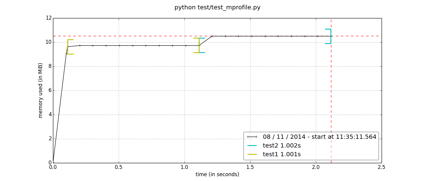
where you can see the memory used (in the y-axis) as a function of time (x-axis). Furthermore, we have used two functions, test1 and test2, and it is possible to see with the colored brackets at what time do these functions start and finish.
This plot was generated with the following simple script:
import time

@profile
def test1():
    n = 10000
    a = [1] * n
    time.sleep(1)
    return a

@profile
def test2():
    n = 100000
    b = [1] * n
    time.sleep(1)
    return b

if __name__ == "__main__":
    test1()
    test2()
what happens here is that we have two functions, test1() and test2() in which we create two lists of different sizes (the one in test2 is bigger). We call time.sleep() for one second so that the function does not return too soon and so we have time to get reliable memory measurements.
The decorator @profile is optional and is useful so that memory_profiler knows when the function has been called so he can plot the brackets indicating that. If you don't put the decorator, the example will work just fine except that the brackets will not appear in your plot.
Suppose we have saved the script as test1.py. We run the script as
where mprof is an executable provided by memory_profiler. If the above command was successful it will print something like this
$ mprof run test1.py
mprof: Sampling memory every 0.1s
running as a Python program...
The above command will create a .dat file on your current working directory, something like mprofile_20141108113511.dat. This file (you can inspect it, it's a text file) contains the memory measurements for your program.
You can now plot the memory measurements with the command
This will open a matplotlib window and show you the plot:
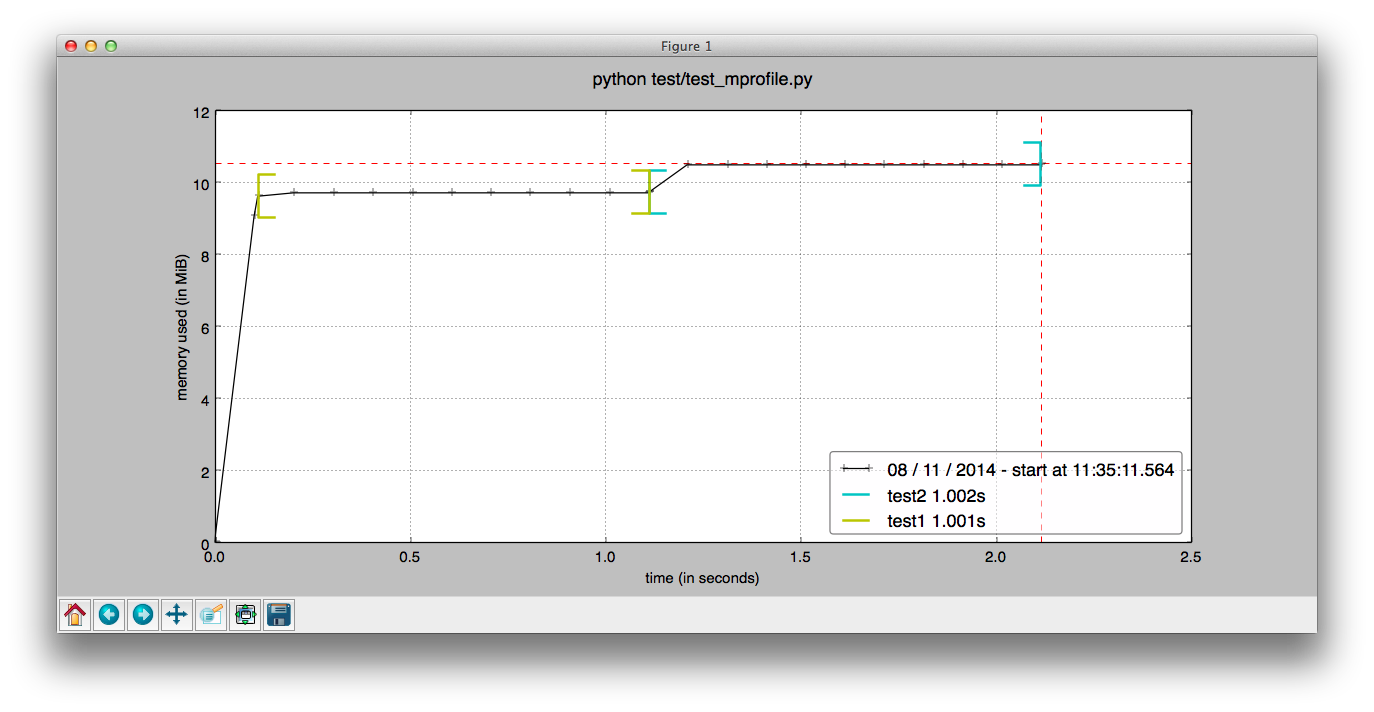
As you see, attention has been paid to the default values so that the plot it generates already looks decent without much effort. The not-so-nice-part is that, at least as of November 2014, if you want to customize the plot, well, you'll have to look and modify the mprof script. Some refactoring is still needed in order to make it easier to customize the plots (work in progress).