











Every metric is based off the following two score functions:
Expenditure can be interpreted as money spent, or tokens, or time required.
I will not give a deep discussion of how to measure the score curves, $s_H$ and $s_A$. There are many practical difficulties involved in this.
I will generally address only scores on a single task; applications to collections of tasks (benchmark scores) can be a bit more complicated.
I will mostly not discuss other desirable properties of metrics - e.g. whether it is understandable, whether it is generalizable.
If score curves are very concave (meaning score is invariant to expenditure) then just reporting the raw score is fine, given some reasonable amount of expenditure.
If score curves show high returns to expenditure then we need a metric that takes into account test-time scaling.
Benchmarking against human abilities helps us generalize to entirely new tasks.
As the models get very good then many of the human-relevant benchmarks become no longer useful.
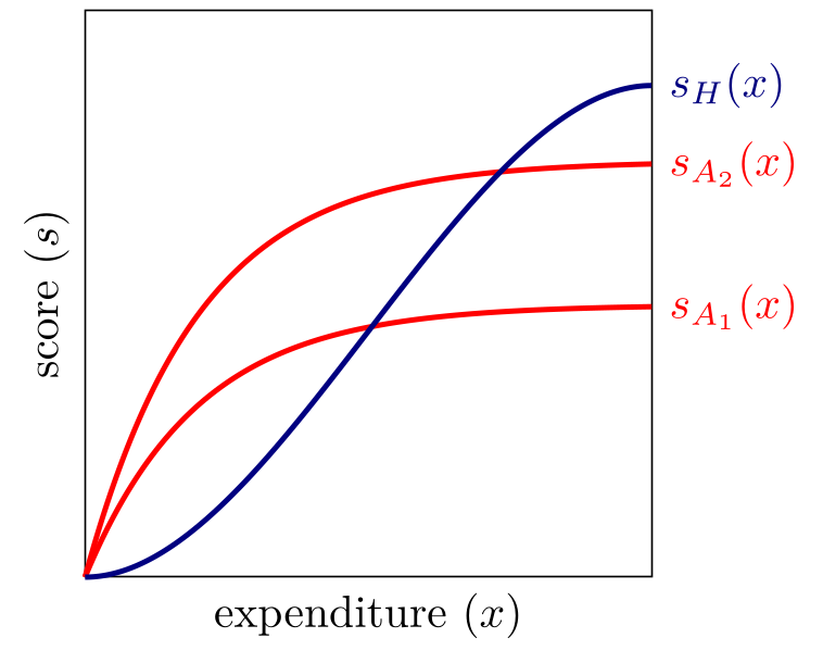
Each agent and each human is characterized by a function from expenditure to score, $s(x)$, and $s^{-1}(\bar{s})$ represents the expenditure required to reach a score $\bar{s}$.
In general I interpret score as performance on a single task, e.g., the speedup on an optimization problem. We could also interpret score as the share of binary tasks completed, or the probability of completing a single task.1
Expenditure will generally be treated as money, but it can also be interpreted as time or tokens.
Human-grounded metrics that compare agent and human expenditure require both expenditures to be measured in the same units or converted into a common unit such as dollars.
I will typically draw the agent curves ($s_A(\cdot)$) as more concave than the human curves ($s_H(\cdot)$).2 I think this accurately represents the reality for most tasks today (e.g., Wijk et al. (2025)), but it could change.
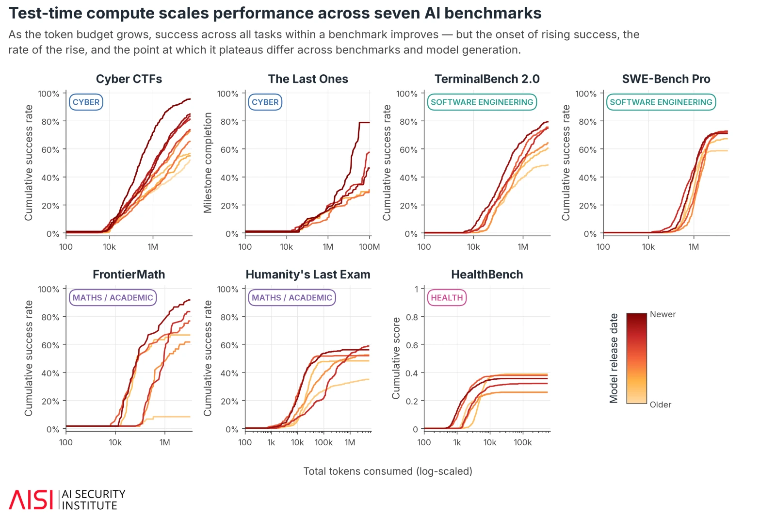
AISI’s recent post on More test-time compute, more capability has a good discussion and visualization of test-time scaling curves across a variety of different benchmarks:
We first discuss metrics that depend only on the agent’s score, without benchmarking against humans.3
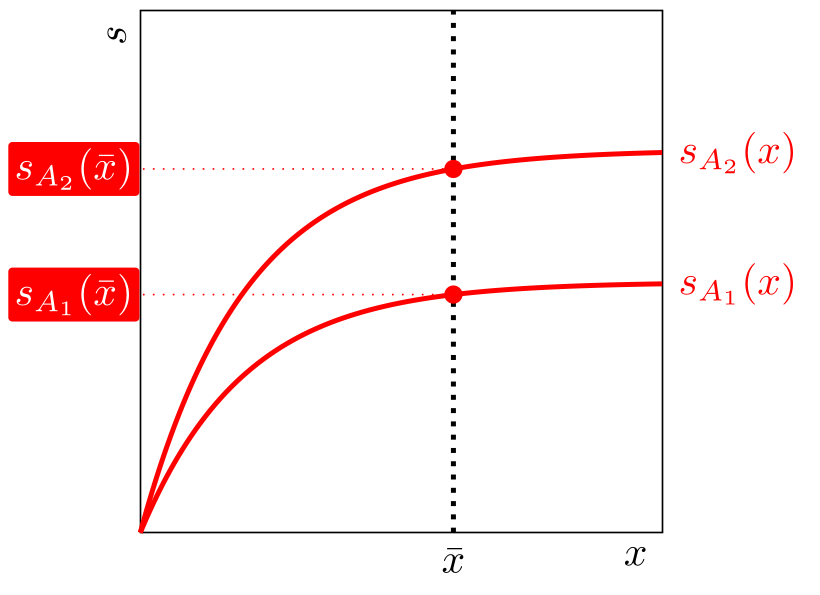
This is the typical way we report most evals: pick a fixed expenditure $\bar{x}$ and report each agent’s score $s_A(\bar{x})$. If $s_A(\cdot)$ reliably asymptotes at a fairly low value of $x$, then this is a sufficient statistic for most purposes.
This metric becomes less useful when agent scores continue increasing even at high levels of expenditure; e.g., see the criticisms by Noam Brown and Kapoor et al. (2025).4
Another reason for fixing expenditure is to increase separation in scores, where a higher level of expenditure would cause saturation, and so little discrimination between model capabilities (e.g. in a recent AISI post).5
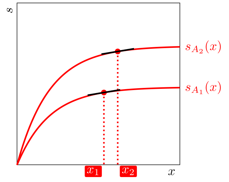
A common practical response is to report the score at the point where the function plateaus, or falls below a certain slope (assuming concavity). E.g., Kwa and West et al. (2025) say “Models were given sufficiently high token limits to reach a plateau in success rate.”
This is equivalent to reporting score at some high expenditure level, representing the highest reasonable level of expenditure. It will not be well-defined if the score function never plateaus.
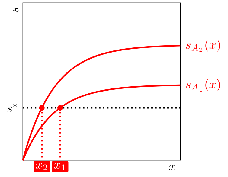
We can instead fix a target score $\bar{s}$ and report the infimum expenditure needed to reach that score: $x=s_{A}^{-1}(\bar{s})$.
This metric will only give a finite number if the evaluated model can achieve the score $\bar{s}$. This is a cost-efficiency metric, often used when looking at declines in model costs over time (Gundlach et al. 2026; Cottier et al. 2025).6
If agents all had the same relative costs of performance, then new generations of models would shift multiplicatively left (additively left in log-space), and this type of “efficiency” metric would be a sufficient statistic for ability. However, there is some reason to believe that new models typically have disproportionate impacts at high expenditures, i.e. they make certain scores available that would have been almost impossible at any expenditure for an earlier model.7
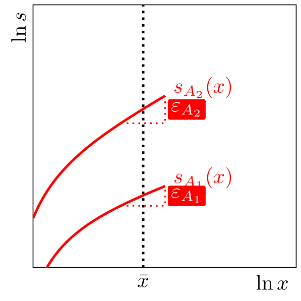
If the returns to expenditure do not plateau, even at significant levels of expenditure, then score at a fixed expenditure is not a satisfactory metric.
Instead, it can be useful for a metric to express the marginal returns to expenditure. The nature of the scaling can vary across domains, and so the appropriate metric is often chosen depending on the shape of the scaling. Two common patterns:
In each case the relationship will be linear on a graph with appropriately transformed axes. However it’s also possible that no consistent relationship exists.
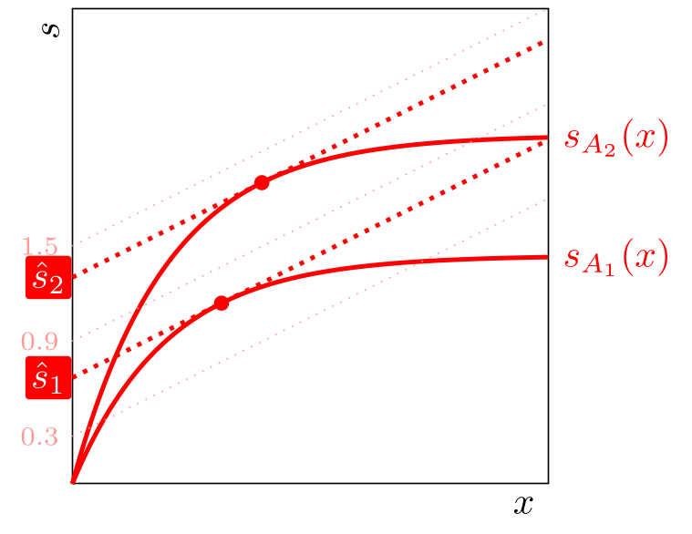
If we are willing to be opinionated about the relative value of expenditure and score, then we can express those tradeoffs with a utility function $U(s,x)$, which will give us a metric of value. Each agent will have a different level of optimal expenditure (represented by a tangency point on the diagram) and a different level of utility.
The utility can be expressed as an expenditure-adjusted score: the score at zero expenditure that would make you indifferent between receiving that score and using the agent at its optimal expenditure:
\[\hat{s}_A:\quad U(\hat{s}_A,0)=\max_{x\geq 0} U(s_A(x),x).\]
The utility can also be expressed in monetary units, representing the total value you get from using the agent. Visually this will be the intersection of the optimal indifference curve with the $x$-axis (not pictured, it would fall on the negative part of the $x$-axis).
\[\hat{x}_A:\quad U(0,-\hat{x}_A)=\max_{x\geq 0} U(s_A(x),x).\]
A natural metric for human expenditure is time spent on the problem, and so some of these metrics use human-equivalent time as a metric of agent capability. However, if we are comparing agent and human expenditure on the same axes, then money is a more natural interpretation of $x$.
Many continuously-scored tasks grade agents by a single human expenditure threshold. E.g. the Opus 5 system card reports a series of AI R&D tasks, and for each a score that was achieved by a human after a specific amount of time (e.g. 8 hours or 40 hours). Agents can then be graded as passing if they beat the baseline.
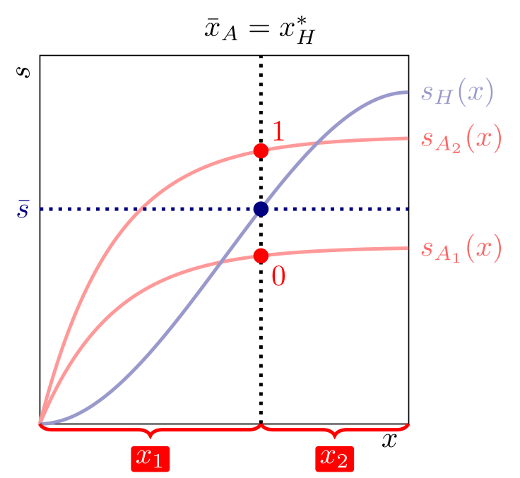
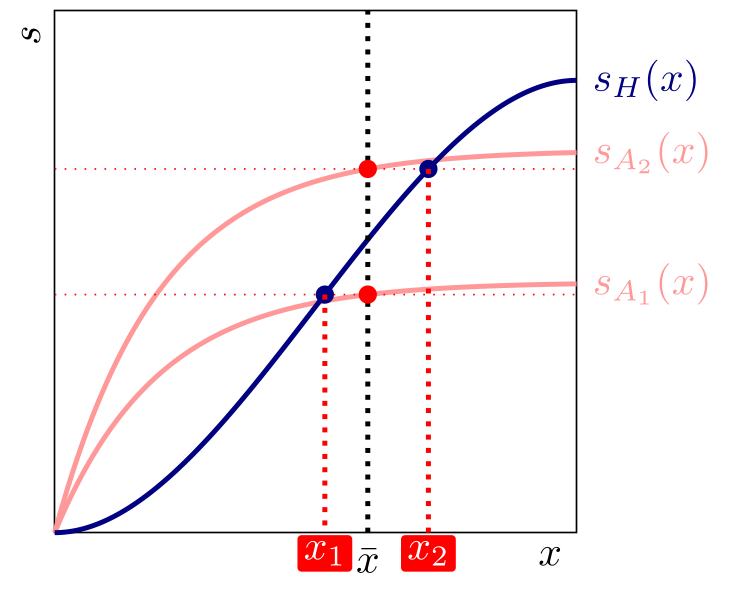
METR’s “time horizon” metric (Kwa and West et al. (2025)) combines many binary scores into a human-equivalent time for each model, based on the $x$ at which the agent matches or exceeds the human score half the time.9
Formally, for each task we choose a reference score \(\bar{s}\) and calculate the infimum human expenditure \(x_H^*=s_H^{-1}(\bar{s})\) needed to achieve that score. Here expenditure is measured in time, but it could also be measured in money.
We then calculate the agent’s score at some fixed expenditure \(\bar{x}_A\), and give the agent a binary score based on whether \(s_A(\bar{x}_A)\) is above or below \(\bar{s}\).
The diagram shows equal expenditure on humans and agents (\(\bar{x}_A=x_H^*\)). The fixed agent expenditure \(\bar{x}_A\) need not equal the human expenditure \(x_H^*\), but equal expenditure on each is a natural choice for interpretability.
We can extend the time horizon metric by retaining the agent’s continuous score rather than reducing it to a binary comparison.
We elicit each agent at a single expenditure level, $\bar{x}_A$, and then compare the resulting score with the whole human curve, rather than with one binary threshold.
The human-equivalent expenditure is $s_H^{-1}(s_A(\bar{x}_A))$: the expenditure at which a human would achieve the same score.
This method is much more statistically efficient than the binary time-horizon method. Reasons to use binary scoring include (1) that it may be difficult to map out the entire $s_H(\cdot)$ function but easier to measure a single point, and (2) that the returns to human effort may look like a step function, e.g., if the score metric $s$ is itself binary.
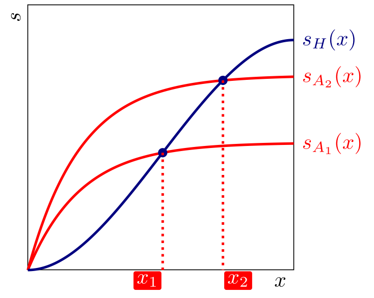
Unlike the fixed-budget metrics, this metric uses the agent’s entire performance curve, making it useful for tasks where we expect significant test-time scaling.
We define the “expenditure horizon” as the supremum of the common expenditures at which the agent matches or beats humans: $\sup\{x\geq 0:s_A(x)\geq s_H(x)\}$.
The expenditure horizon does not provide a finite crossing point if agents dominate humans at every level of expenditure.
Expenditure horizon can also be unstable if the slopes of $s_H$ and $s_A$ are similar.
Cunningham et al. (2026) introduce this metric, based in part on the apple-picking model (Cunningham and Shetty 2026).10
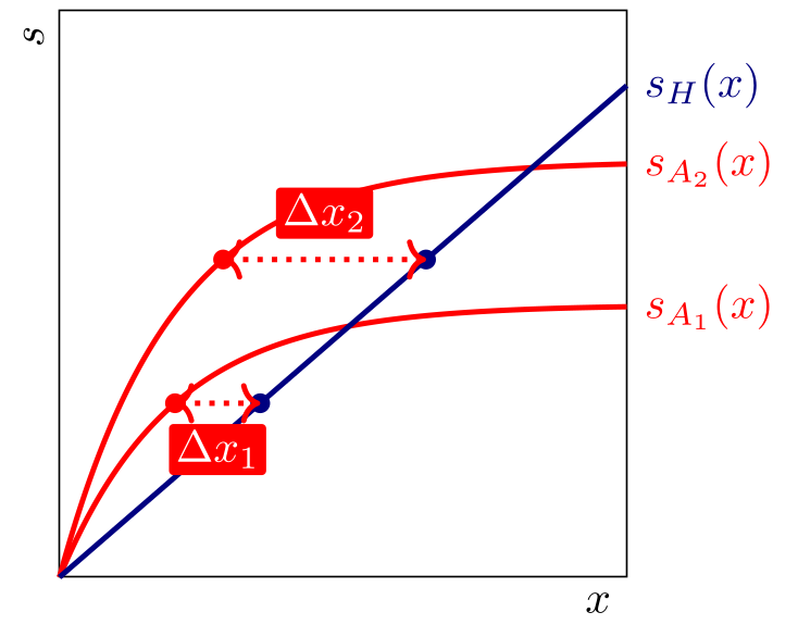
We can also directly measure the effective cost-saving relative to using a human on a task.
For simplicity we draw the human score curve as linear. We can then identify the point at which the marginal returns to expenditure are equal between agents and humans (assuming concave returns to expenditure on agents). If you are allocating budget between agents and humans then this will be the point at which you switch from spending on agents to spending on humans.
This point also identifies the economic value: the horizontal distance between the red and blue points represents the expenditure saving due to using an agent:
\[\Delta x_{A_i}=\max_{x\geq 0}\\{s_H^{-1}(s_{A_i}(x))-x\\}.\]
This applies the utility framework discussed above, but now our indifference curves are determined by the returns to human labor (our outside option).
This is discussed further in Cunningham et al. (2026) and Cunningham and Shetty (2026).
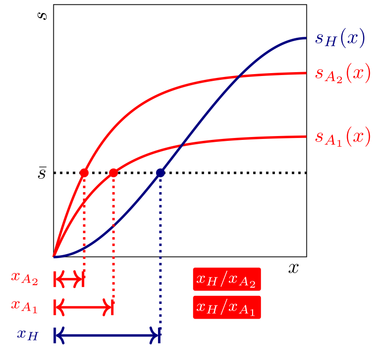
An alternative metric is to simply compare the cost of achieving some fixed score, $\bar{s}$. In the figure, $x_{A_i}=s_{A_i}^{-1}(\bar{s})$ and $x_H=s_H^{-1}(\bar{s})$:
\[\text{human-relative cost}_{A_i}(\bar{s})= \frac{s_H^{-1}(\bar{s})}{s_{A_i}^{-1}(\bar{s})} =\frac{x_H}{x_{A_i}}.\]
This metric is consistent across values of $\bar{s}$ when the human and agent score curves differ only by a multiplicative horizontal rescaling.
Unlike the other metrics in this section, this metric remains useful when agents strictly dominate humans (i.e. the red curve is entirely to the left of the blue curve).
Two related papers incorporate model and human costs in different ways (both are somewhat different from a true hybrid: they use a rule-based allocation of tasks between agents and humans):
Erol et al. (2025) define a model’s cost-of-pass on problem $p$ as $v(m,p)=C_m(p)/R_m(p)$: the cost of one attempt divided by its probability of success, or equivalently the expected cost of obtaining a correct answer under independent retries. Their frontier cost-of-pass chooses the cheapest available model or qualified human expert separately for each problem:
\[V_p(\mathcal M\cup\mathcal M_0)=\min\left\lbrace\min_{m\in\mathcal M}v(m,p),\,v(\mathrm{expert},p)\right\rbrace.\]Thus, the frontier can use a human for tasks on which human labor is cheaper and a model for tasks on which inference is cheaper; its average over a task distribution measures the cost of assigning each task to the cheaper producer.13 This combines humans and models through task-by-task routing rather than within-task collaboration.
Patwardhan et al. (2025) (GDPval) describe speed-and-cost metrics that combine model win rates with the time and cost of model generation, expert review, and human rework.14
Thanks to Beth Barnes, Manish Shetty, Nate Rush, Thomas Kwa, Parker Whitfill, Megan Kinniment, Alexander Barry, and Kaivu Hariharan for helpful discussions and feedback.
Alomrani, Mohammad Ali, Yingxue Zhang, Derek Li, et al. 2025. Reasoning on a Budget: A Survey of Adaptive and Controllable Test-Time Compute in LLMs. https://arxiv.org/pdf/2507.02076.pdf.
Bartz-Beielstein, Thomas, Carola Doerr, Daan van den Berg, et al. 2020. Benchmarking in Optimization: Best Practice and Open Issues. https://arxiv.org/pdf/2007.03488.pdf.
Brown, Bradley, Jordan Juravsky, Ryan Ehrlich, et al. 2024. Large Language Monkeys: Scaling Inference Compute with Repeated Sampling. https://arxiv.org/abs/2407.21787.
Cottier, Ben, Ben Snodin, David Owen, and Tom Adamczewski. 2025. LLM Inference Prices Have Fallen Rapidly but Unequally Across Tasks. https://epoch.ai/data-insights/llm-inference-price-trends.
Cunningham, Tom, and Manish Shetty. 2026. “An Apple-Picking Model of AI R&D.” March 13. https://tecunningham.github.io/posts/2026-03-13-apple-picking-ai.html.
Cunningham, Tom, Manish Shetty, Vincent Cheng, and Nate Rush. 2026. “Expenditure Horizon: Measuring Optimization Ability, with an Application to NanoGPT.” METR, July 21. https://metr.org/blog/2026-07-21-expenditure-horizon/#appendix-d.
Erol, Mehmet Hamza, Batu El, Mirac Suzgun, Mert Yuksekgonul, and James Zou. 2025. Cost-of-Pass: An Economic Framework for Evaluating Language Models. https://arxiv.org/abs/2504.13359.
Fogelson, Alex, Zachary A. Brown, Hans Gundlach, Jayson Lynch, and Neil Thompson. 2026. Two AI Metrics Diverged: Will It Make All the Difference? https://arxiv.org/pdf/2607.00913.pdf.
Folkerts, Linus, Will Payne, Simon Inman, et al. 2026. Measuring AI Agents’ Progress on Multi-Step Cyber Attack Scenarios. https://arxiv.org/abs/2603.11214.
Gundlach, Hans, Jayson Lynch, Matthias Mertens, and Neil Thompson. 2026. The Price of Progress: Price Performance and the Future of AI. https://arxiv.org/abs/2511.23455.
Jones, Charles I. 1995. “R&D-Based Models of Economic Growth.” Journal of Political Economy 103 (4): 759–784. https://doi.org/10.1086/262002.
Kapoor, Sayash, Benedikt Stroebl, Zachary S. Siegel, Nitya Nadgir, and Arvind Narayanan. 2025. “AI Agents That Matter.” Transactions on Machine Learning Research. https://arxiv.org/abs/2407.01502.
Kwa, Thomas, Ben West, Joel Becker, et al. 2025. “Measuring AI Ability to Complete Long Tasks.” arXiv Preprint arXiv:2503.14499, ahead of print. https://doi.org/10.48550/arXiv.2503.14499.
McFadyen, Jessica, Ole Jorgensen, Harry Coppock, Kevin Wei, and Cozmin Ududec. 2026. How Inference Compute Shapes Frontier LLM Evaluation. https://arxiv.org/abs/2606.17930.
OpenAI. 2026. “An OpenAI Model Has Disproved a Central Conjecture in Discrete Geometry.” May 20. https://openai.com/index/model-disproves-discrete-geometry-conjecture/.
Patwardhan, Tejal, Rachel Dias, Elizabeth Proehl, et al. 2025. GDPval: Evaluating AI Model Performance on Real-World Economically Valuable Tasks. https://arxiv.org/abs/2510.04374.
Wijk, Hjalmar, Tao Lin, Joel Becker, et al. 2025. RE-Bench: Evaluating Frontier AI R&D Capabilities of Language Model Agents Against Human Experts. https://arxiv.org/abs/2411.15114.
此内容由惯性聚合(RSS阅读器)自动聚合整理,仅供阅读参考。 原文来自 — 版权归原作者所有。