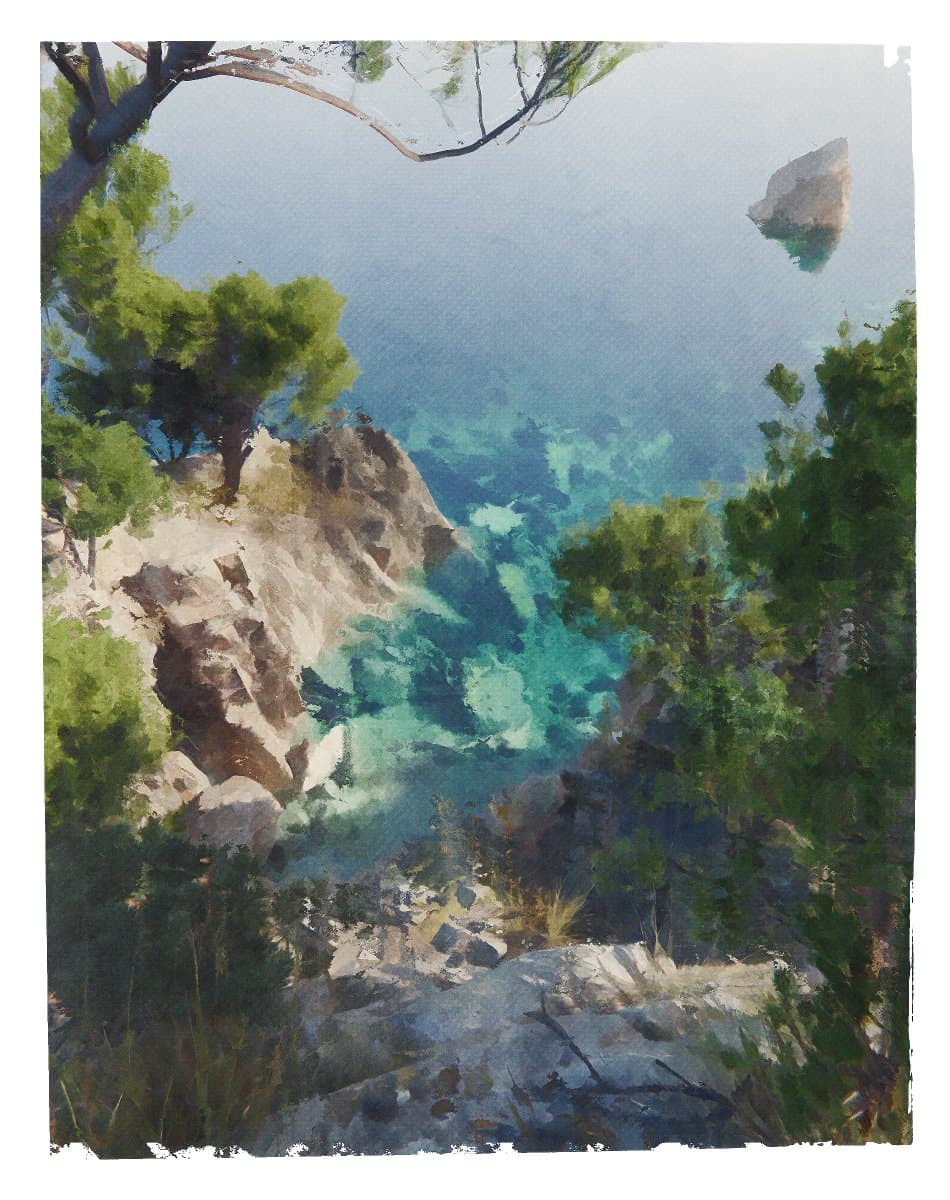
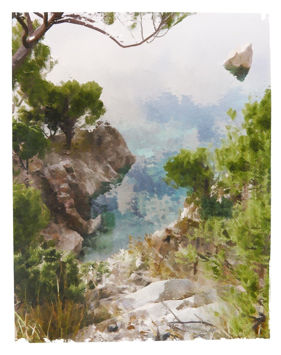
Writing a shader that can reproduce the look and feel of aquarelle, watercolor, or gouache to obtain a more painterly output for my WebGL scenes has always been a long-term goal of mine. Inspired by the work of very talented 3D artists such as @simonxxoo or @arpeegee, the contrast between paintings and the added dimension allowed by 3D renderers was always very appealing to me. On top of that, my recent work with stylized shaders to mimic the hand-drawn Moebius art style emphasized not only that obtaining such stylized output was possible but also that post-processing was more likely than not the key to emulating any artistic style.
After several months of on/off research that frankly was not leading to much, I stumbled upon a smoothing filter I never heard about before: the Kuwahara filter. Lucky for me, it turned out that many (very smart) people published papers about it and its ability to transform any image input into a painting-like work of art. By implementing it into a custom post-processing pass and going through many ups and downs in the process, I got very close to my original objective by building what is essentially a real-time 3D painting running in the browser:
This article is the culmination of months of work, trial and error, and research to craft the perfect painterly shader for your next WebGL project. In it, we will deep dive into the characteristics of the Kuwahara filter that make it so great at transforming our work into paintings, as well as look into several techniques highlighted in the many papers I read to improve the original implementation and have it return a sharper, and more anisotropic output. Finally, we'll go through a bit of color correction and the use of textures to achieve a satisfying and accurate painting effect.
Up until then, my only attempts at painterly shader consisted of several implementations of custom materials focused on emulating specific aspects of paint that I instinctively listed as essential to get a convincing output:
The absence of texture/normal detail
Preserved edges
Quantized colors
Below is an example of one of my "best" iterations from that exploratory work. It notably uses a Voronoi noise to smudge normals and a paintbrush texture for a more realistic look and feel.
However, despite my best efforts, this work was dead in the water as my implementation was severely flawed and only worked with a subset of meshes. From then on, I knew I had to go the post-processing route to solve most of those issues, but I didn't know how. Then, one day, I stumbled upon the beautiful work of @arpeegee, who gave me the keywords I was missing all this time: Kuwahara filter.
Originally intended to remove noise through smoothing from medical images, the Kuwahara filter is most commonly used today to transform any input into stylistic paintings through post-processing.
Unlike other smoothing filters that reduce noise but also, on the way, blur our edges, the Kuwahara filter is capable of preserving edges and corners. That specificity is what makes it so good at achieving painting-like artistic effects by getting us two crucial visual properties of paintings:
The smoothing erases some of the texture details.
The filter preserves the edges and, in some cases, increases the sharpness compared to the original input.
It achieves this by executing the following steps on each pixel of our input, which in our case would be our underlying 3D scene:
We center a box around a pixel.
We divide the box into 4 "sub-boxes" or Sectors.
We calculate the average color and variance for each Sector.
We set our pixel to the average color of the Sector with the lowest variance.
I built the widget below to visually represent those sectors surrounding a given pixel at work:
You can see by selecting the edge examples that:
when a pixel sits just outside an edge, the Sector with the lowest variance will always be outside the edge
when a pixel sits just inside an edge, the Sector with the lowest variance will be inside the edge
highlighting the edge-preserving capabilities of this filter.
The widget below showcases how this process of picking the average color of the Sector with the lowest variance impacts an entire image:
Notice how, with a reasonable kernel size, we maintain the overall shapes featured in the underlying image but erase many details like, in this case, transparency. However, we can also observe that with a higher kernel size, the image filter, unfortunately, falls apart and denatures quite drastically our input, indicating that we will have to strike the right balance between kernel size and the strength of our painterly post-processing effect.
Now that we have a good understanding of the inner workings of the Kuwahara filter, let's implement it as a post-processing effect on top of a React Three Fiber scene. Much like the work done in Moebius-style post-processing and other stylized shaders, we will define our custom post-processing pass using the Pass class from the post-processing package.
This post-processing pass will:
Take our underlying scene as an input.
Implement the Kuwahara filter in its fragment shader.
Output the resulting scene.
The implementation of it in GLSL goes as follows:
Implementation of the Kuwahara filter in GLSL
4
uniform sampler2D inputBuffer;
5
uniform vec4 resolution;
6
uniform sampler2D originalTexture;
10
void getSectorVarianceAndAverageColor(vec2 offset, int boxSize, out vec3 avgColor, out float variance) {
11
vec3 colorSum = vec3(0.0);
12
vec3 squaredColorSum = vec3(0.0);
13
float sampleCount = 0.0;
16
for (int y = 0; y < boxSize; y++) {
17
for (int x = 0; x < boxSize; x++) {
18
vec2 sampleOffset = offset + vec2(float(x), float(y));
19
vec3 color = sampleColor(sampleOffset);
21
squaredColorSum += color * color;
27
avgColor = colorSum / sampleCount;
28
vec3 varianceRes = (squaredColorSum / sampleCount) - (avgColor * avgColor);
29
variance = dot(varianceRes, vec3(0.299, 0.587, 0.114));
33
vec3 boxAvgColors[SECTOR_COUNT];
34
float boxVariances[SECTOR_COUNT];
36
getSectorVarianceAndAverageColor(vec2(-kernelSize, -kernelSize), kernelSize, boxAvgColors[0], boxVariances[0]);
37
getSectorVarianceAndAverageColor(vec2(0, -kernelSize), kernelSize, boxAvgColors[1], boxVariances[1]);
38
getSectorVarianceAndAverageColor(vec2(-kernelSize, 0), kernelSize, boxAvgColors[2], boxVariances[2]);
39
getSectorVarianceAndAverageColor(vec2(0, 0), kernelSize, boxAvgColors[3], boxVariances[3]);
41
float minVariance = boxVariances[0];
42
vec3 finalColor = boxAvgColors[0];
44
for (int i = 1; i < SECTOR_COUNT; i++) {
45
if (boxVariances[i] < minVariance) {
46
minVariance = boxVariances[i];
47
finalColor = boxAvgColors[i];
51
gl_FragColor = vec4(finalColor, 1.0);
In the code featured above, we can see that:
We're allocating an array of vec3 and float to store the average color and variance for each of our Sectors, respectively.
We're computing those stats by sampling the color for every pixel in a given Sector along the x-axis and y-axis and calculating the average and variance using the formulas we saw in the previous part.
We then set minVariance and finalColor as the variance and average color of the first Sector by default.
We then loop through the other Sectors to find the Sector with the lowest variance and set its corresponding average color as the output of our fragment shader.
Doing this will result in a version of our scene with fewer texture details while preserving the overall shape of our geometries and also introducing artifacts that look somewhat like brush strokes:
Through our initial implementation of the Kuwahara filter as a custom post-processing pass, we already achieved a somewhat convincing paint effect. However, it suffers from several drawbacks at high kernel sizes that may make our underlying scene not discernable by the viewer, and the appearance of our "brush strokes" could most likely be improved.
Ideally, we could fix both these issues in one go by allowing larger kernel sizes for a more intense stylized effect for our scene and also have more natural-looking artifacts with a slight tweak of our Kuwahara filter. That is what Giuseppe Papari proposes in his paper Artistic Edge and Corner Enhancing Smoothing. In it, he presents an extension to the Kuwahara filter that:
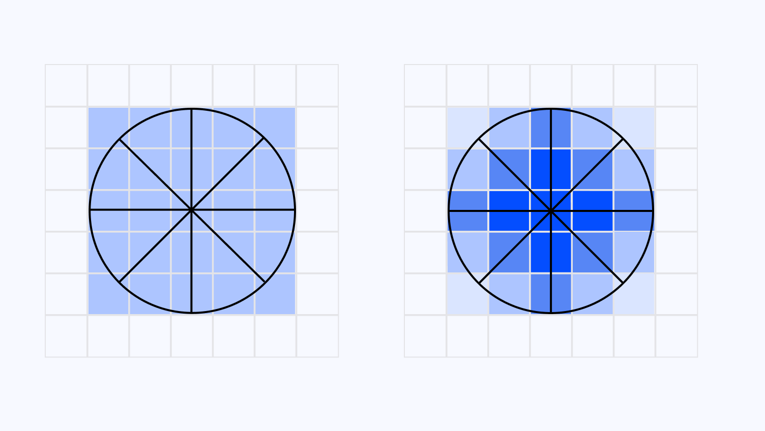
Removes the square-shaped kernel in favor of a circular one.
Improves the weight influence that each pixel has on the filter.
In this part, we will implement some of those improvements with an additional section on potential performance improvements. It may sound absurd but; I like my paintings to run as close to 60fps as possible.
A circular-shaped kernel allows us to increase the number of Sectors when evaluating the color of a given pixel. Its box-shaped counterpart can only allow for up to four Sectors making more complex edge lines not well-preserved. Through his experiments, Papari found that eight Sectors were the ideal amount to balance output quality and good performance.
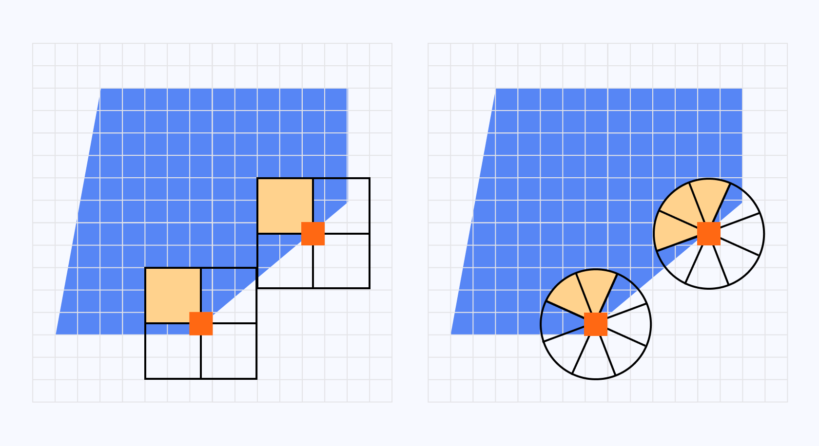
The widget below showcases the impact that this subtle modification in the implementation of our filter has on a simple image:
Here, we can see that, compared to what we observed in the first part, this version of the Kuwahara filter yields a way better output even at a larger kernel size! The circular shape and the higher number of Sectors allow us to preserve edge lines for more complex angles and patterns.
We can tweak the fragment shader code to implement Papari's circular kernel into our post-processing pass by modifying the parts that compute variance and average color by Sector:
Switching to a circular kernel in our Kuwahara filter implementation
3
void getSectorVarianceAndAverageColor(float angle, float radius, out vec3 avgColor, out float variance) {
4
vec3 colorSum = vec3(0.0);
5
vec3 squaredColorSum = vec3(0.0);
6
float sampleCount = 0.0;
8
for (float r = 1.0; r <= radius; r += 1.0) {
9
for (float a = -0.392699; a <= 0.392699; a += 0.196349) {
10
vec2 sampleOffset = r * vec2(cos(angle + a), sin(angle + a));
11
vec3 color = sampleColor(sampleOffset);
13
squaredColorSum += color * color;
19
avgColor = colorSum / sampleCount;
20
vec3 varianceRes = (squaredColorSum / sampleCount) - (avgColor * avgColor);
21
variance = dot(varianceRes, vec3(0.299, 0.587, 0.114));
26
vec3 sectorAvgColors[SECTOR_COUNT];
27
float sectorVariances[SECTOR_COUNT];
29
for (int i = 0; i < SECTOR_COUNT; i++) {
30
float angle = float(i) * 6.28318 / float(SECTOR_COUNT);
31
getSectorVarianceAndAverageColor(angle, float(radius), sectorAvgColors[i], sectorVariances[i]);
In the end, the filter's principle is roughly the same. What changes here is which pixel is picked for a given sector and included in the average and variance.
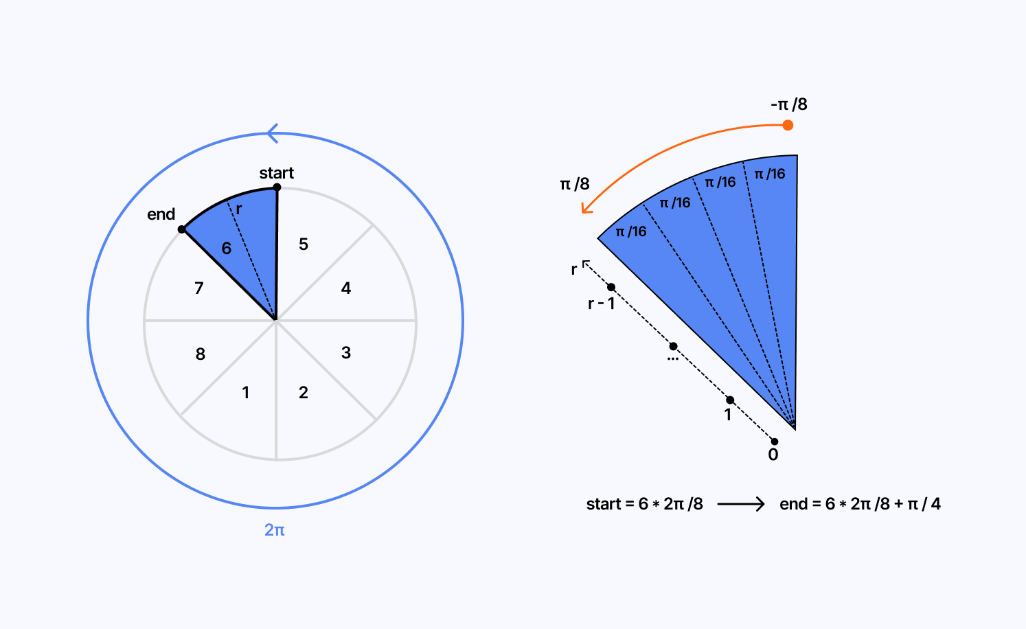
The demo below uses this extended version of the Kuwahara filter on top of our scene. It lets us use a larger kernel size, yielding a more stylized output while keeping our scene discernable:
The artifacts left by the filter are still quite visible at large kernel sizes. According to Papari's study, this effect is due to the weighting of the colors when calculating the average and the variance of a given Sector, as it does not discriminate any pixel. If a pixel is in a sector, it contributes the same amount to the calculations.
Using Gaussian weights fixes this issue:
It provides a gradual fall-off from the center of the Sector to its edges.
This results in more natural-looking transitions from one Sector to another, thus avoiding abrupt changes that would otherwise make those artifacts very visible.
It emphasizes the central pixels more likely to represent the most accurate sector color, giving them more importance when calculating the average color.
To use Gaussian weighting in our filter, we only need to change a few lines from the previous implementation:
Using Gaussian weighting in our Kuwahara filter implementation
3
float gaussianWeight(float distance, float sigma) {
4
return exp(-(distance * distance) / (2.0 * sigma * sigma));
7
void getSectorVarianceAndAverageColor(float angle, float radius, out vec3 avgColor, out float variance) {
8
vec3 weightedColorSum = vec3(0.0);
9
vec3 weightedSquaredColorSum = vec3(0.0);
10
float totalWeight = 0.0;
12
float sigma = radius / 3.0;
14
for (float r = 1.0; r <= radius; r += 1.0) {
15
for (float a = -0.392699; a <= 0.392699; a += 0.196349) {
16
vec2 sampleOffset = r * vec2(cos(angle + a), sin(angle + a));
17
vec3 color = sampleColor(sampleOffset);
18
float weight = gaussianWeight(length(sampleOffset), sigma);
20
weightedColorSum += color * weight;
21
weightedSquaredColorSum += color * color * weight;
22
totalWeight += weight;
27
avgColor = weightedColorSum / totalWeight;
28
vec3 varianceRes = (weightedSquaredColorSum / totalWeight) - (avgColor * avgColor);
29
variance = dot(varianceRes, vec3(0.299, 0.587, 0.114));
As we can see in the code snippet above:
We compute the weight using the Gaussian formula.
We then take the resulting weight into account when calculating our weighted color sum and weighted squared color sum.
Those weights are then reflected in the final result of the variance and average color for each Sector.
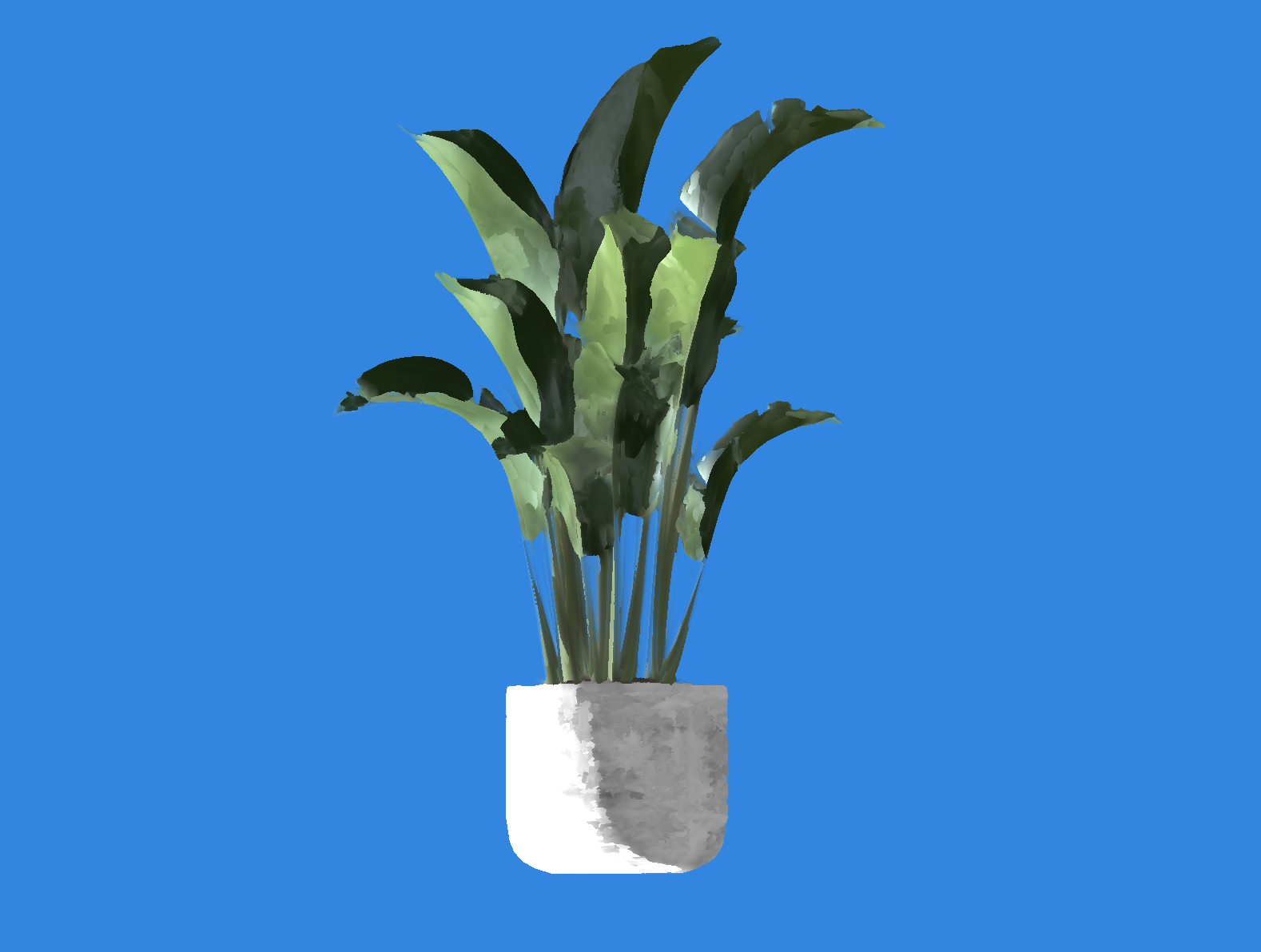
Now, you may wonder whether adding all those nitty-gritty improvements to a filter that already performed quite well is worth it. You can see the result for yourself in the comparison below between a frame of our first scene using the original implementation of the Kuwahara filter and one using the Papari extension:
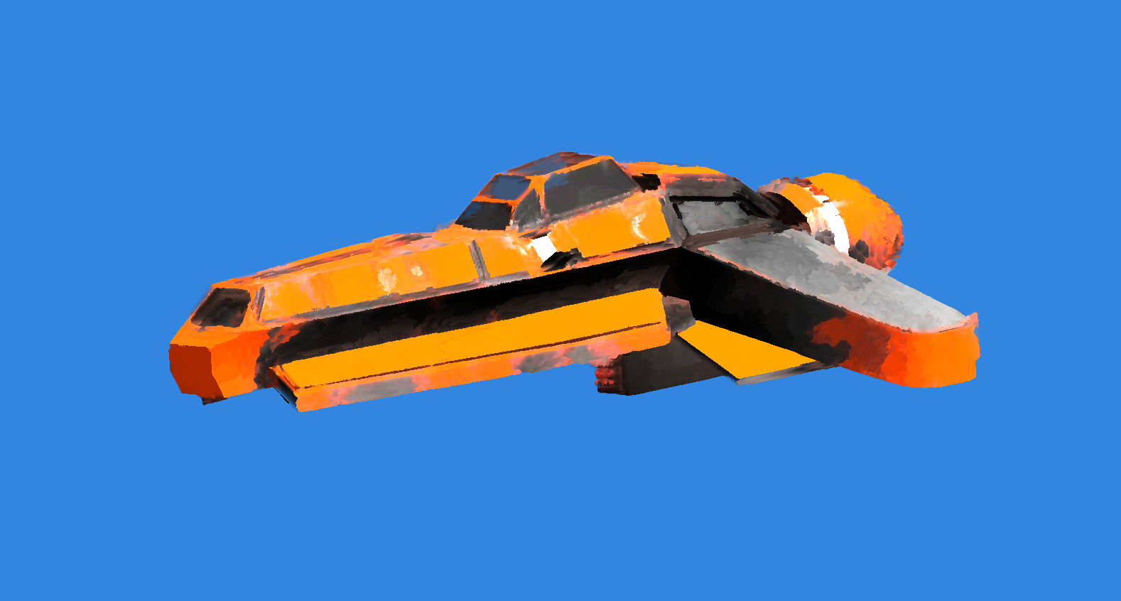
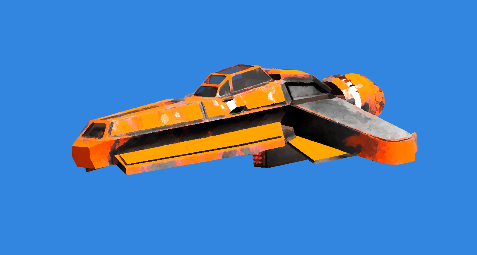
The result looks already better than previously, even at a low kernel size! Let's observe now the difference between both implementations for a higher value:
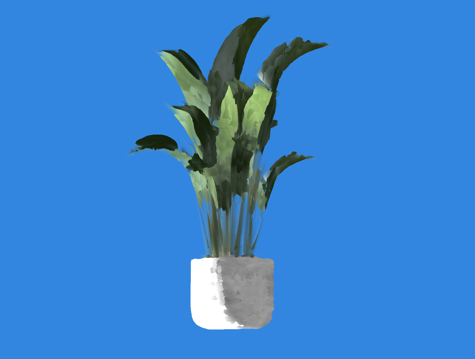
The Gaussian function used to calculate the weights of our pixel is, unfortunately, quite expensive to run, even more so in all those nested loops necessary to sample each pixel of a given Sector. This improvement is costing us a lot of frames, and it would be very tempting to disregard it and revert to the original weighting method.
However, a team of smart individuals found a way to squeeze more performance out of the filter while maintaining the advantages given by the Gaussian. In Anisotropic Kuwahara Filtering with PolynomialWeighting Functions, they propose to replace the Gaussian with a polynomial that roughly approximates it.
[(x + ζ) − ηy^2]^2
Using Polynomial weighting in our Kuwahara filter implementation
3
float polynomialWeight(float x, float y, float eta, float lambda) {
4
float polyValue = (x + eta) - lambda * (y * y);
5
return max(0.0, polyValue * polyValue);
8
void getSectorVarianceAndAverageColor(float angle, float radius, out vec3 avgColor, out float variance) {
9
vec3 colorSum = vec3(0.0);
10
vec3 squaredColorSum = vec3(0.0);
11
float weightSum = 0.0;
16
for (float r = 1.0; r <= radius; r += 1.0) {
17
for (float a = -0.392699; a <= 0.392699; a += 0.196349) {
19
vec2 sampleOffset = vec2(r * cos(angle + a), r * sin(angle + a));
20
vec3 color = sampleColor(sampleOffset);
21
float weight = polynomialWeight(sampleOffset.x, sampleOffset.y, eta, lambda);
When trying out this formula, I noticed the performance improvements highlighted in the paper but also that I could get a satisfying output at a smaller kernel size compared to what we've implemented so far. I'm still not exactly sure why 🤷♂️, but I'll take it.
Papari's extension of the Kuwahara filter is already a step towards a lovely painterly shader, however, (I must sound like a broken record at this point) we still can perceive some artifacts left by the filter on the resulting scene. Indeed, the painting effect is applied indiscriminately to the input without any consideration for the overall structure of the current frame. In the case of a true painting, the artist would adapt the flow of the brush based on the direction of the edge. We're not getting this here.
Luckily, Anisotropic Kuwahara Filtering with PolynomialWeighting Functions answers this problem by building upon the concepts of the extended Kuwahara filter we just saw.
In this paper, the authors suggest that we could adapt our circular kernel to the local features of the input during sampling by squeezing and rotating it, thus letting us sample our Sectors more accurately. As a result, our kernel would look more like an ellipsis rather than a circle.
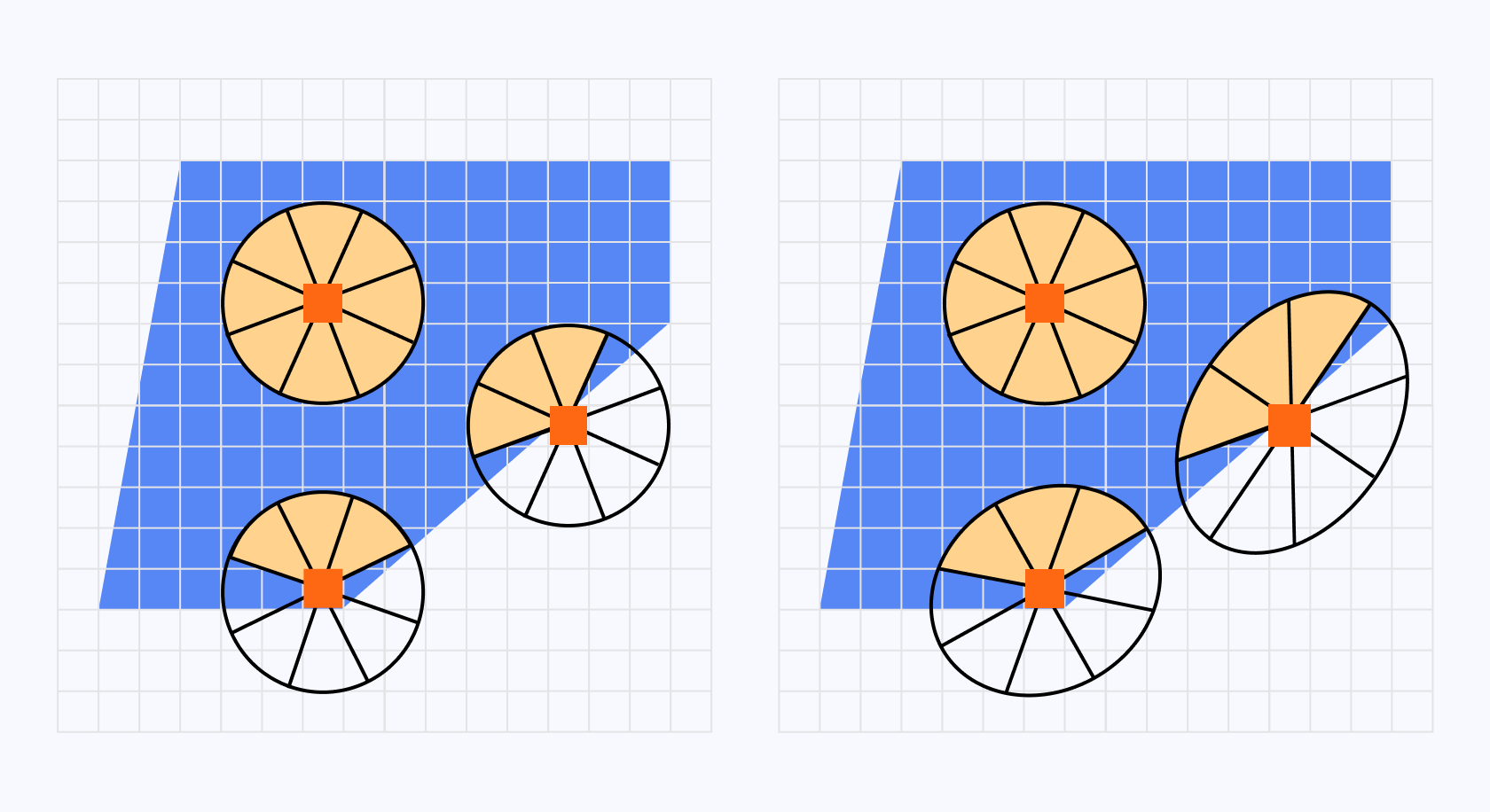
Implementing this improvement will require us to follow several steps and make our post-processing effect multi-pass:
The first pass will take the underlying scene as input and return the structure of the scene.
Then based on this structure as input we'll apply our Kuwahara filter to the underlying scene.
Finally, we'll add one extra pass to apply some tone mapping and other details that will make our painterly shader shine.
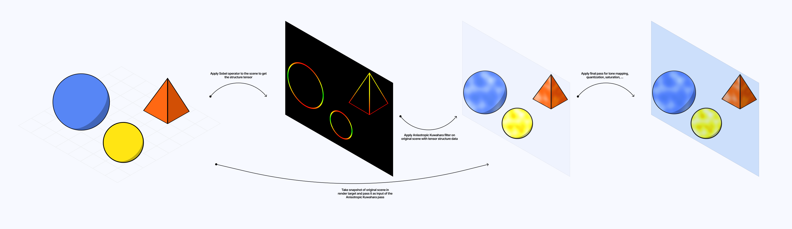
To obtain the structure of our scene, we can leverage a Sobel operator which I introduced in Moebius-style post-processing and other stylized shaders earlier this year.
Sx = [[-1, 0, 1], [-2, 0, 2], [-1, 0, 1]]
Sy = [[-1, -2, -1], [0, 0, 0], [1, 2, 1]]
However, this time we won't use it for edge detection like we did back then. We will apply our Sobel Matrix for every pixel but instead of a rapid change in intensity, which is characteristic of edges, we want to extract the partial derivatives along the x/y axis representing the rate of change.
Applying our Sobel Matrices when sampling
2
uniform sampler2D inputBuffer;
3
uniform vec4 resolution;
6
const mat3 Gx = mat3( -1, -2, -1, 0, 0, 0, 1, 2, 1 );
7
const mat3 Gy = mat3( -1, 0, 1, -2, 0, 2, -1, 0, 1 );
9
vec4 computeStructureTensor(sampler2D inputTexture, vec2 uv) {
10
vec3 tx0y0 = texture2D(inputTexture, uv + vec2(-1, -1) / resolution.xy).rgb;
11
vec3 tx0y1 = texture2D(inputTexture, uv + vec2(-1, 0) / resolution.xy).rgb;
12
vec3 tx0y2 = texture2D(inputTexture, uv + vec2(-1, 1) / resolution.xy).rgb;
13
vec3 tx1y0 = texture2D(inputTexture, uv + vec2( 0, -1) / resolution.xy).rgb;
14
vec3 tx1y1 = texture2D(inputTexture, uv + vec2( 0, 0) / resolution.xy).rgb;
15
vec3 tx1y2 = texture2D(inputTexture, uv + vec2( 0, 1) / resolution.xy).rgb;
16
vec3 tx2y0 = texture2D(inputTexture, uv + vec2( 1, -1) / resolution.xy).rgb;
17
vec3 tx2y1 = texture2D(inputTexture, uv + vec2( 1, 0) / resolution.xy).rgb;
18
vec3 tx2y2 = texture2D(inputTexture, uv + vec2( 1, 1) / resolution.xy).rgb;
With those partial derivatives, we can obtain a structure tensor
In the following fragment shader code, we apply both Sobel matrices at a given pixel, compute the structure tensor, and return it as an output.
Using Sobel Matrices to obtain the structure tensor
2
uniform sampler2D inputBuffer;
3
uniform vec4 resolution;
6
const mat3 Gx = mat3( -1, -2, -1, 0, 0, 0, 1, 2, 1 );
7
const mat3 Gy = mat3( -1, 0, 1, -2, 0, 2, -1, 0, 1 );
10
vec4 computeStructureTensor(sampler2D inputTexture, vec2 uv) {
11
vec3 tx0y0 = texture2D(inputTexture, uv + vec2(-1, -1) / resolution.xy).rgb;
12
vec3 tx0y1 = texture2D(inputTexture, uv + vec2(-1, 0) / resolution.xy).rgb;
13
vec3 tx0y2 = texture2D(inputTexture, uv + vec2(-1, 1) / resolution.xy).rgb;
14
vec3 tx1y0 = texture2D(inputTexture, uv + vec2( 0, -1) / resolution.xy).rgb;
15
vec3 tx1y1 = texture2D(inputTexture, uv + vec2( 0, 0) / resolution.xy).rgb;
16
vec3 tx1y2 = texture2D(inputTexture, uv + vec2( 0, 1) / resolution.xy).rgb;
17
vec3 tx2y0 = texture2D(inputTexture, uv + vec2( 1, -1) / resolution.xy).rgb;
18
vec3 tx2y1 = texture2D(inputTexture, uv + vec2( 1, 0) / resolution.xy).rgb;
19
vec3 tx2y2 = texture2D(inputTexture, uv + vec2( 1, 1) / resolution.xy).rgb;
21
vec3 Sx = Gx[0][0] * tx0y0 + Gx[1][0] * tx1y0 + Gx[2][0] * tx2y0 +
22
Gx[0][1] * tx0y1 + Gx[1][1] * tx1y1 + Gx[2][1] * tx2y1 +
23
Gx[0][2] * tx0y2 + Gx[1][2] * tx1y2 + Gx[2][2] * tx2y2;
25
vec3 Sy = Gy[0][0] * tx0y0 + Gy[1][0] * tx1y0 + Gy[2][0] * tx2y0 +
26
Gy[0][1] * tx0y1 + Gy[1][1] * tx1y1 + Gy[2][1] * tx2y1 +
27
Gy[0][2] * tx0y2 + Gy[1][2] * tx1y2 + Gy[2][2] * tx2y2;
29
return vec4(dot(Sx, Sx), dot(Sy, Sy), dot(Sx, Sy), 1.0);
33
vec4 tensor = computeStructureTensor(inputBuffer, vUv);
35
gl_FragColor = tensor;
If we were to visualize our scene with this tensor pass applied on top, this is what we'd obtain:
Thanks to the Structure Tensor we just obtained, we can derive the information we need to adapt our filter to the local features of our scene. This process is rather tedious and involves some notions of linear algebra that can seem daunting at first. Thus, we'll proceed step-by-step and avoid taking unnecessary shortcuts.
We want to know in which direction a given pixel points towards, i.e. the dominant direction and orientation of the tensor at a given position. Luckily, there is a mathematical concept that represents just that: eigenvalues and eigenvectors.
Through our structure tensor, we'd like to obtain λ1 and derive its corresponding eigenvector, giving us the dominant direction of the local structure, to adapt our filter.
We can do so by starting from the definition of an eigenvector A * v = λ * v. Given a Matrix [[a, b], [b,c]], we have:
A * v = λ * v
A * v - λ * v = 0
A * v - λ * I * v where I is the identity matrix
(A - λ * I) * v = 0
Since we established that v is non-null, the only way for a product of a matrix transformation and non-zero vector to be null is if the transformation completely squishes space. This can be represented by a zero determinant for that matrix transformation, hence det(A - λ * I) = 0
det([[a - λ, b], [b, d - λ]]) = 0
By applying the formula of the determinant we highlighted above we get: (a - λ) * (d - λ) - b^2 = 0
Finally, if we simplify this equation, we get the following quadratic equation to solve for lambda: λ^2 - (a + d)λ + (ad - b^2) = 0
The solution of this quadratic equation gives us two possible values for lambda as we expected:
λ = [(a + d) ± √((a + d)^2 - 4*(ad - b^2))] / 2
Doing all these steps in our fragment shader code would be relatively intensive. If you look a bit closer at the formula above, you will notice that we can replace some bits with the ones of the determinant and the trace of the transformation matrix:
λ = [trace ± √(trace² - 4*determinant)] / 2
thus making us not have to perform all the steps we just went through in our shader code: we can directly use this formula to compute both eigenvalues.
Computing the eigenvalues of our structuretensor
1
float Jxx = structureTensor.r;
2
float Jyy = structureTensor.g;
3
float Jxy = structureTensor.b;
5
float trace = Jxx + Jyy;
6
float determinant = Jxx * Jyy - Jxy * Jxy;
8
float lambda1 = trace * 0.5 + sqrt(trace * trace * 0.25 - determinant);
9
float lambda2 = trace * 0.5 - sqrt(trace * trace * 0.25 - determinant);
Now that we have our eigenvalues, we can pick the largest one to derive our eigenvector following this definition:
(A - λ * I) * v = 0
[Jxx - λ, Jxy] [vx] = [0] and [Jxy, Jyy - λ]* [vy] [0]
(Jxx - λ) * vx + Jxy * vy = 0 and Jxy * vx + (Jyy - λ) * vy = 0
vx = -Jxy * vy / (Jxx - λ), and by setting vy to 1 for simplicity we get: vx = -Jxy / (Jxx - λ)
we can then multiply both components by Jxx - λ and obtain the final value for our eigenvector: v = (-Jxy, Jxx - λ)
We can use it as is in our code, however, through many rounds of trial and error, I had to resort to using this eigenvector only if Jxy relative to the other components of the tensor matrix was above zero.
Computing the eigenvector of our structure tensor
1
vec4 getDominantOrientation(vec4 structureTensor) {
2
float Jxx = structureTensor.r;
3
float Jyy = structureTensor.g;
4
float Jxy = structureTensor.b;
6
float trace = Jxx + Jyy;
7
float determinant = Jxx * Jyy - Jxy * Jxy;
9
float lambda1 = trace * 0.5 + sqrt(trace * trace * 0.25 - determinant);
10
float lambda2 = trace * 0.5 - sqrt(trace * trace * 0.25 - determinant);
12
float jxyStrength = abs(Jxy) / (abs(Jxx) + abs(Jyy) + abs(Jxy) + 1e-7);
16
if (jxyStrength > 0.0) {
17
v = normalize(vec2(-Jxy, Jxx - lambda1));
22
return vec4(normalize(v), lambda1, lambda2);
From the Structure Tensor of our underlying scene, we derived both its eigenvalues and eigenvector. We could have also merely headed over to Anisotropic image segmentation by a gradient structure tensor to find those formulas, however, we're grown-ups and it's nice to step out of our comfort zone to learn how to derive/define the tools and formulas we use in our shaders from time to time 🙂.
In Anisotropic Kuwahara Filtering with PolynomialWeighting Functions, the authors define the anisotropy A using those eigenvalues as follows:
gg
With this formula, we can derive that:
A ranges from 0 to 1
when λ1 = λ2, the anisotropy is 0, representing a isotropic region.
when λ1 > λ2, the anisotropy tends towards 1, representing an anisotropic region.
With the anisotropy now defined, we can use it to shape the circular kernel from the Kuwahara filter along the x-axis and y-axis with
Excentricity of the circular kernel
4
vec4 structureTensor = texture2D(inputBuffer, vUv);
6
vec3 sectorAvgColors[SECTOR_COUNT];
7
float sectorVariances[SECTOR_COUNT];
9
vec4 orientationAndAnisotropy = getDominantOrientation(structureTensor);
10
vec2 orientation = orientationAndAnisotropy.xy;
12
float anisotropy = (orientationAndAnisotropy.z - orientationAndAnisotropy.w) / (orientationAndAnisotropy.z + orientationAndAnisotropy.w + 1e-7);
15
float scaleX = alpha / (anisotropy + alpha);
16
float scaleY = (anisotropy + alpha) / alpha;
Notice how:
As the anisotropy approaches 1, the ellipsis becomes more elongated along the x-axis, stretching our circular kernel.
When we have a relatively isotropic region, the scale factors are 1 resulting in our kernel remaining circular.
We now know how to stretch and scale our kernel based on the anisotropy, the remaining task we need to achieve is to orient it accordingly using the eigenvector we computed previously and defining a rotation matrix from it.
Adapt our kernel using anisotropy and the eigenvector from our structure tensor
3
void getSectorVarianceAndAverageColor(mat2 anisotropyMat, float angle, float radius, out vec3 avgColor, out float variance) {
4
vec3 weightedColorSum = vec3(0.0);
5
vec3 weightedSquaredColorSum = vec3(0.0);
6
float totalWeight = 0.0;
11
for (float r = 1.0; r <= radius; r += 1.0) {
12
for (float a = -0.392699; a <= 0.392699; a += 0.196349) {
13
vec2 sampleOffset = r * vec2(cos(angle + a), sin(angle + a));
14
sampleOffset *= anisotropyMat;
24
vec4 structureTensor = texture2D(inputBuffer, vUv);
26
vec3 sectorAvgColors[SECTOR_COUNT];
27
float sectorVariances[SECTOR_COUNT];
29
vec4 orientationAndAnisotropy = getDominantOrientation(structureTensor);
30
vec2 orientation = orientationAndAnisotropy.xy;
32
float anisotropy = (orientationAndAnisotropy.z - orientationAndAnisotropy.w) / (orientationAndAnisotropy.z + orientationAndAnisotropy.w + 1e-7);
35
float scaleX = alpha / (anisotropy + alpha);
36
float scaleY = (anisotropy + alpha) / alpha;
38
mat2 anisotropyMat = mat2(orientation.x, -orientation.y, orientation.y, orientation.x) * mat2(scaleX, 0.0, 0.0, scaleY);
40
for (int i = 0; i < SECTOR_COUNT; i++) {
41
float angle = float(i) * 6.28318 / float(SECTOR_COUNT);
42
getSectorVarianceAndAverageColor(anisotropyMat, angle, float(radius), sectorAvgColors[i], sectorVariances[i]);
As you can see above, the last step simply consists of applying this matrix to our sampleOffset. Voilà! We adapted our Kuwahara filter to be anisotropic!
I acknowledge that this process is rather tedious, however, the techniques described in the paper about the anisotropic Kuwahara filter that we reimplemented here are interesting and demonstrate the power that a few matrix transformations can have on an image and all the information we can derive from these.
The result in itself is subtle, and you'll mostly notice the advantages when:
analyzing some specific and complex details of your scene from up close once the filter is applied
having a very high kernel size
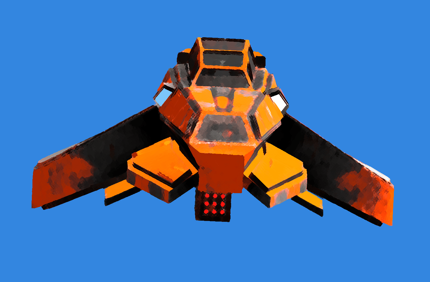
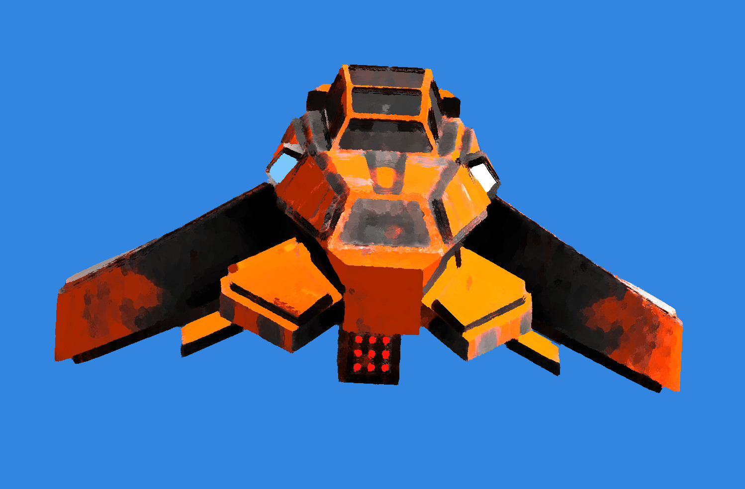
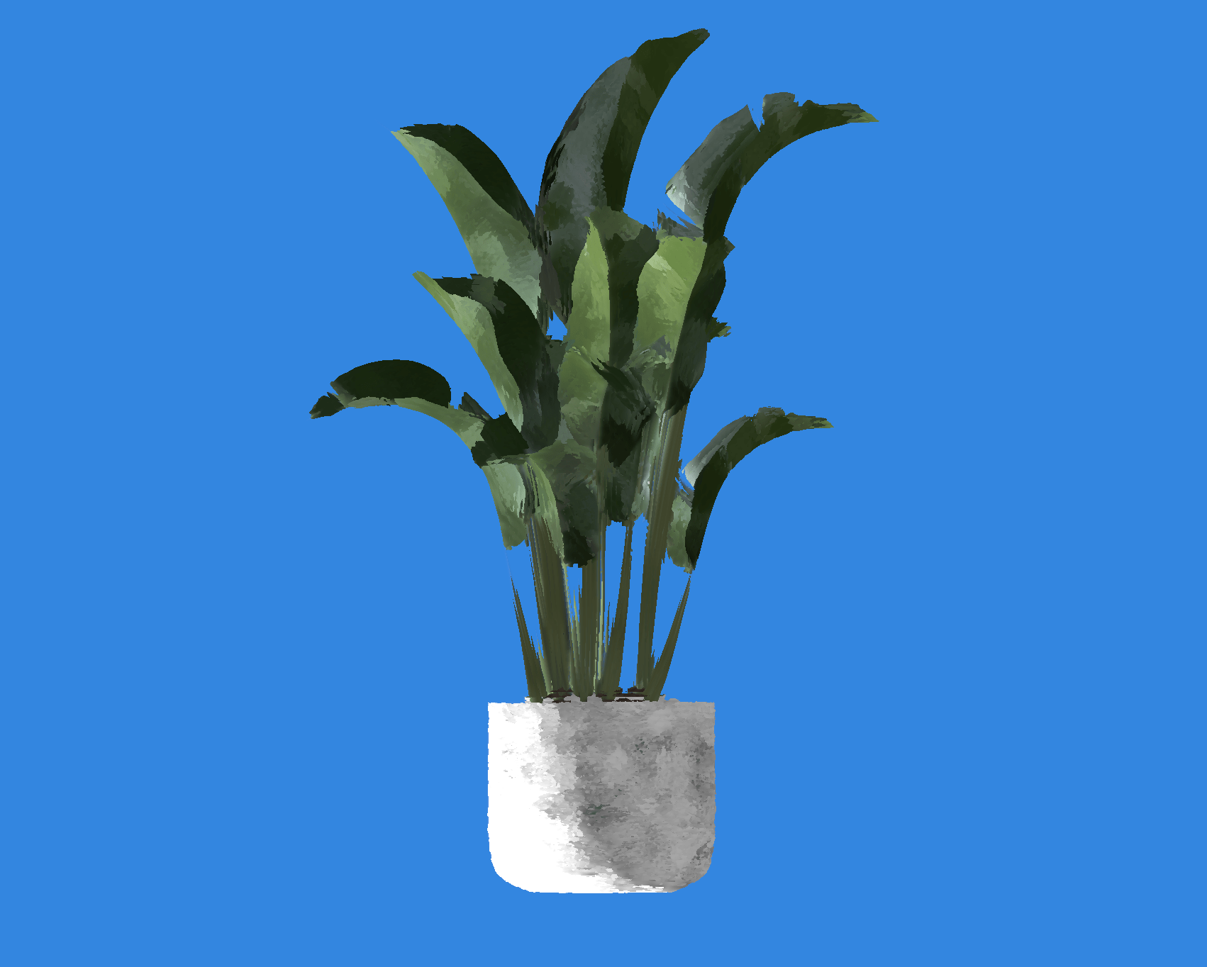
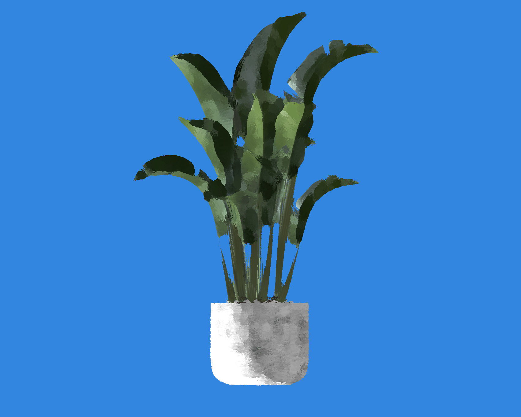
Below is the full implementation of our multi-pass anisotropic Kuwahara filter:
To bring out the best of our painterly shader, we can add a final post-processing pass to our scene to perform a few tweaks such as:
quantization
color interpolation
saturation
tone mapping
adding some texture to the output
Quantization will help reduce the number of colors our output will feature. I covered this method in length in The Art of Dithering and Retro Shading for the Web. As a reminder, the formula behind quantization is:
floor(color * (n - 1) + 0.5)/n - 1 where n is the total number of colors.
In our fragment shader for our final pass, we can add quantization by:
Calculating the grayscale value of the current pixel.
Setting the number of colors n. In my examples, I picked 16.
Using the formula established above.
Clamp the range to avoid extreme values which wouldn't yield a realistic painting effect.
Applying quantization in our final post-processing pass
2
vec3 color = texture2D(inputBuffer, vUv).rgb;
3
vec3 grayscale = vec3(dot(color, vec3(0.299, 0.587, 0.114)));
8
float qn = floor(x * float(n - 1) + 0.5) / float(n - 1);
9
qn = clamp(qn, 0.2, 0.7);
On top of that, to obtain a more painterly color output, we can use a Two Point Interpolation to blend our colors with our grayscale quantized image:
For a darker quantized pixel, we'd opt to interpolate from black (or close to black) to the image color based on that quantization value.
For a lighter quantized pixel, we'd interpolate from the image to white.
Adding two point color interpolation
4
color = mix(vec3(0.1), color.rgb, qn * 2.0);
6
color = mix(color.rgb, vec3(1.0), (qn - 0.5) * 2.0);
This method emphasizes the contrast between light (represented by white space) and dark areas (more painted, darker colors).
To make our output pop more, I also chose to increase the saturation of our colors:
Saturating our color output
3
vec3 sat(vec3 rgb, float adjustment) {
4
vec3 W = vec3(0.2125, 0.7154, 0.0721);
5
vec3 intensity = vec3(dot(rgb, W));
6
return mix(intensity, rgb, adjustment);
11
color = sat(color, 1.5);
And, finally, I added some tone mapping for better color balance:
Applying tone mapping to our scene
9
return clamp((x * (a * x + b)) / (x * (c * x + d) + e), 0.0, 1.0);
16
color = sat(color, 1.5);
17
color = ACESFilm(color);
19
vec4 outputColor = vec4(color, 1.0);
20
gl_FragColor = outputColor;
You can see that these little color improvements compound into significant changes highlighting the best features of our painterly shader:
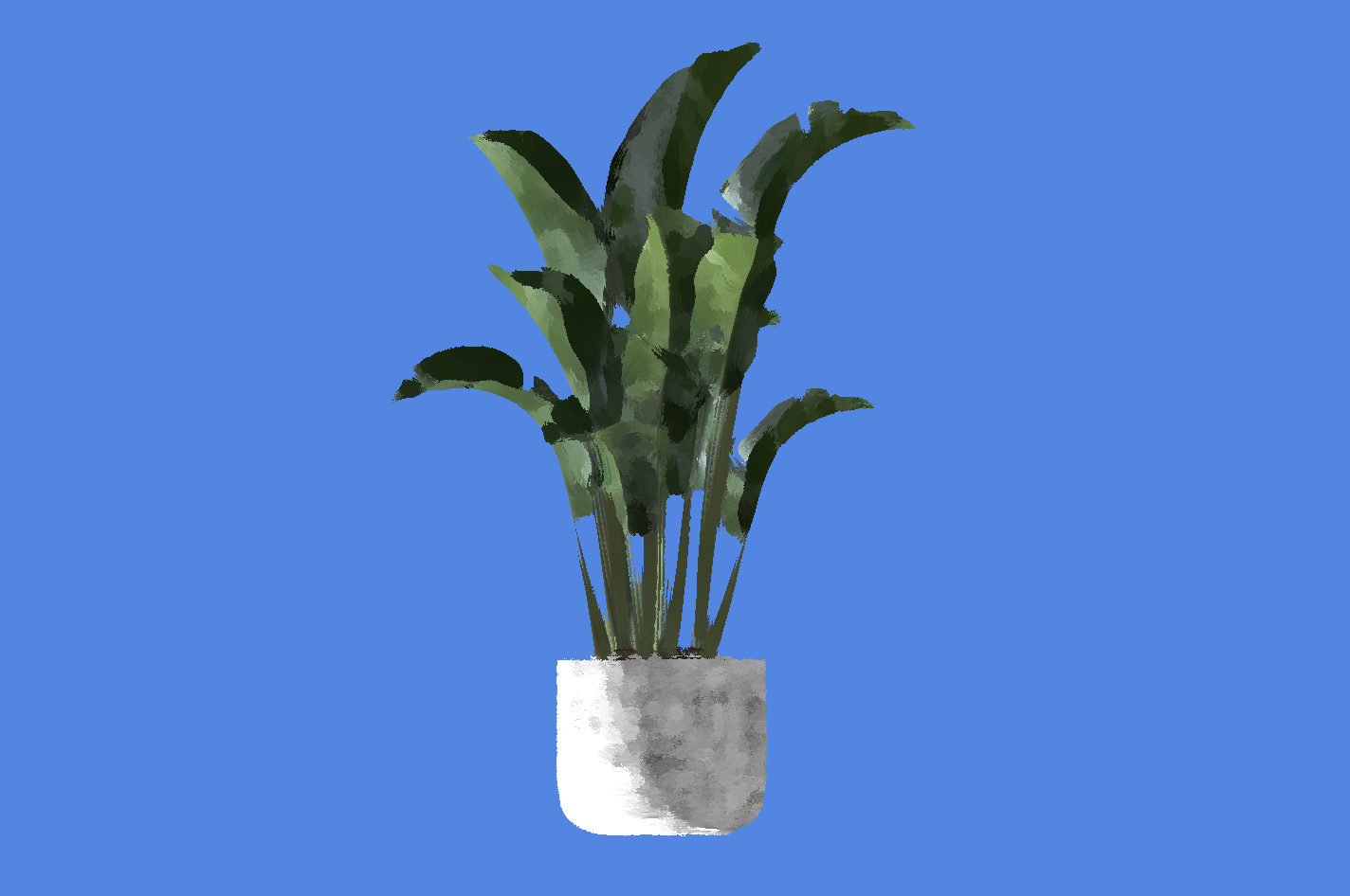
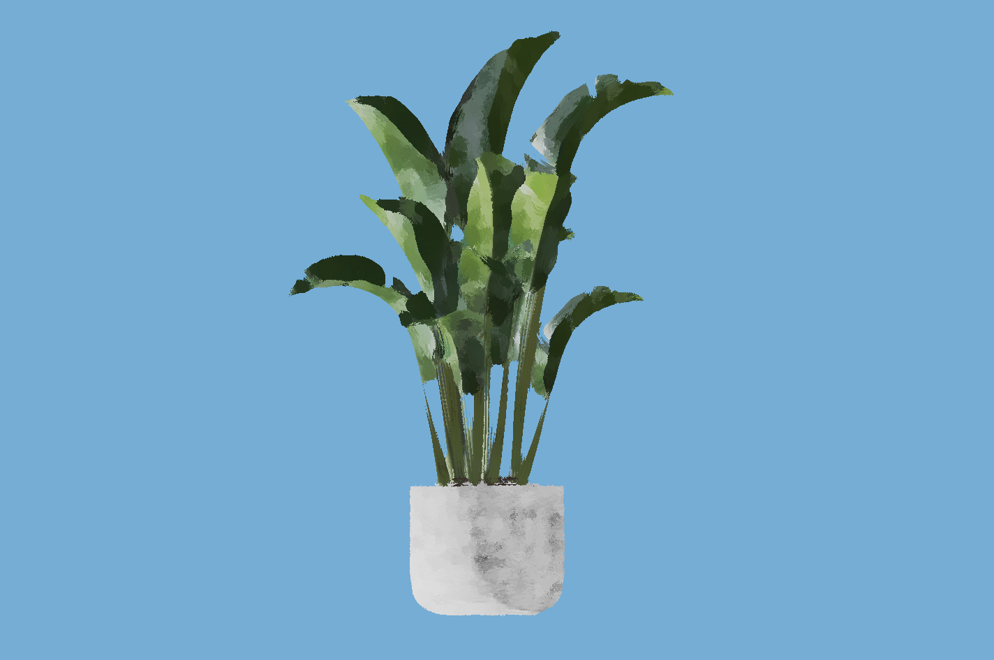
To wrap it all up, and give our output some physicality and realism, we can add a paper-like texture and blend it with the color output of our fragment shader, exactly as @arpeegee did in the example that originally inspired this article. This is a very easy trick that adds a lot of details to our scene and makes it look like a real painting.
The demo below bundles all those improvements together on top of the anisotropic Kuwahara filter making an otherwise standard scene look like a beautiful painting with many features reminiscent of watercolor which is the effect I was originally trying to achieve.
As we saw throughout this article, making a satisfying painterly shader seemed simple on the surface thanks to the standard implementation of the Kuwahara filter. However, it turned out to be much more intricate once we started to dig deeper and trying to fix the artifacts that each technique yielded. If you were to ask me my take on the topic, I'd consider the Papari extension of the Kuwahara filter with polynomial weighting to be enough in most cases, while also being relatively performant compared to its anisotropic counterpart. At the end of the day, it's almost more a question of personal taste/creative choice as the different iterations of this image filter can produce drastically different results given an underlying scene/image.
Nonetheless, deep diving into how to obtain the structure tensor of an image and deriving anisotropy through many layers of linear algebra is far from useless as the technique can be ported to many other post-processing effects (one of which I'm considering writing about here). Consider it as one additional tool in your ever-growing shader toolbelt.
To finish this article, which was quite the undertaking not going to lie, here are a couple more shots/paintings of some of the test scenes I used while building this custom post-processing shader:
此内容由惯性聚合(RSS阅读器)自动聚合整理,仅供阅读参考。 原文来自 — 版权归原作者所有。