








Richard Startin
Richard Startin is a Senior Software Engineer at Datadog. A version of this post was originally published on his blog.
It can be hard to figure out why response times are high in Java applications. In my experience, when engineers investigate this type of issue, they typically use one of two methods: They either apply a process of elimination to find a recent commit that might have caused the problem, or they use profiles of the system to look for the cause of value changes in relevant metrics.
Both of these approaches are problematic. Making guesses about recent commits can be frustrating for a number of reasons, but mostly because even if you pinpoint the causal change, you still might not know why the change was bad. This leaves you in a kind of limbo, awaiting the recurrence of a problem you can neither understand nor prevent.
In theory, using a profiler makes root cause analysis a part of the triage process, so adopting continuous profiling should make this whole process easier. However, using profilers can be frustrating because engineers typically use the wrong type of profile for analysis. Lots of profiling data focuses on CPU time, but the cause of your latency problem may be related to time spent off CPU instead.
This post is about Datadog’s Java wallclock profiler, which I worked on last year to help address this kind of problem. In the following sections, I will explore how you can use this profiler to improve request latency without making any code changes—or without even seeing the code, for that matter.
Suppose you have metrics that show you that request latency is too high for a particular endpoint. Here is the endpoint-level latency timeseries for a slow endpoint, GET /allocation-stalls (whose name may create a sense of foreboding), in a very contrived demo Java application.
The response time is about 3–4 seconds, which you would like to improve somehow without undertaking an entire R&D project. Unless you have detailed tracing, you might start diagnosing the issue by looking at profiles. OpenJDK has a built-in profiler called Java Flight Recorder (JFR), which Datadog has used historically for collecting CPU profiles from Java services. Here’s what a flame graph of JFR’s jdk.ExecutionSample events looks like after being processed by Datadog’s profiling backend:
At the extreme left-hand side, you can observe JVM activity derived from JFR’s garbage collection (GC) events. Next to that, there are some stack traces for Jetty’s routing (see JettyHandler.doHandle()). To the right are stack traces for handling the requests in another thread pool (see ThreadPoolExecutor$Worker.run()). There’s not much context beyond the frame names, and the most we have to go on is JavaServer.lambda\$allocationStall\$28(), which we can probably guess is related to handling GET /allocation-stalls requests by its name.
Java code can be very generic, and though it’s not always straightforward to map frames to context by frame names alone, in this case it’s easy enough. Expanding the span gets us to where I think most people turn away from profiling, whenever it is as easy to find the relevant frame as it is in this contrived example:
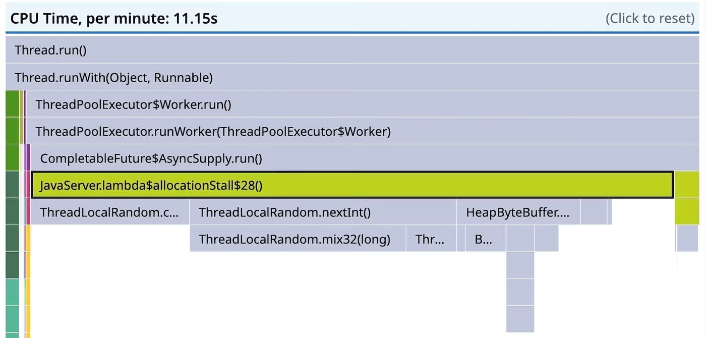
This points to random number generation being the bottleneck, which you aren’t likely to speed up. You may be able to reduce the number of random numbers generated, but in this contrived example, this would require renegotiating requirements. Part of the problem is that this flame graph doesn’t show the complete picture. Without having the full picture, we can’t be sure we know what the bottleneck is, and we might just be looking at the frame we happen to measure the most.
This is where async-profiler comes in.
Some time ago, Datadog started experimenting with using async-profiler instead of JFR’s execution sampler in its Continuous Profiler product. There were two primary motivations for doing this:
So async-profiler’s excellent codebase gave us a starting point for implementing some of the features we had in mind. Below is a flame graph of the same application as above recorded with Datadog’s customization of async-profiler. Notice the Z Garbage Collector (ZGC) activity to the left and compare it to the GC activity we could infer from JFR above. There’s more detail, and it’s more obvious that the service has a GC problem.
Having access to the source code has made it possible to add new fields to event types, such as correlation identifiers. Decorating samples with span IDs makes it possible to link each sample to the endpoint being served, rather than guess based on the frame name (which only gets harder outside of contrived examples). This makes it possible to filter the flame graph by endpoint, instead of merely guessing based on the frame names:
The green frames to the left, which are Java Native Interface (JNI) calls into the lz4-java library, are missing from the JFR flame graph. This is because JFR won’t unwind stacks when the JVM is executing native code. In this particular case, this doesn’t actually distort the flame graph much because LZ4 compression is very fast and doesn’t need as much CPU time as the random number generation we already know about. However, if it were the other way around, the JFR flame graph would be very misleading.
Even though the flame graph now shows a complete picture of CPU time, it still points towards optimizing random number generation, which we can’t do. The problem is now that CPU time isn’t always enough to understand latency.
As used in Datadog’s profiler, async-profiler’s CPU profiler uses CPU time to schedule sampling, which means time spent off-CPU will not be sampled. In Java Thread terms, a CPU profiler can only sample threads in the RUNNABLE state, and it ignores threads in the BLOCKED, TIMED_WAITING, and WAITING states. In contrast, a wallclock profiler can sample threads in any state.
Async-profiler also has a wallclock profiler, but my team and I found that we needed to tailor it to our requirements. Read on for more details.
The first issue we encountered was with overhead. (This problem applies just to our own particular requirements, so don’t be discouraged from using async-profiler’s wallclock profiler in a different context.) CPU profiling is always very lightweight because the overhead is proportional to the number of cores, whereas for wallclock profiling, overhead scales with the number of threads. Async-profiler’s wallclock profiler samples sets of up to eight threads round-robin, and keeping the sampling interval consistent as the number of threads changes will adjust the sampling interval to as low as 100 microseconds. Unless the user provides a thread filter expression to control how many threads to sample, the overhead of this approach can be quite high. Using a predefined thread filter assumes the user knows where the problems are ahead of time, which might be the case when doing offline/non-continuous profiling. It can also produce quite large recordings: In 60 seconds we might record as many as 4.8 million samples, which, at about 64 bytes per JFR event, corresponds to about 250MiB.
We wanted smaller recordings and needed to be very conservative about overhead, so we changed the way threads were sampled. We implemented reservoir sampling of threads so that we could take a uniform sample of a fixed number of threads at a constant sampling interval. This gives a much more manageable upper bound on overhead and recording size: In 60 seconds we can sample 16 threads at 100Hz and record at most 96,000 samples, which is just under 6MiB of JFR events. It should be noted that, when the number of threads changes over time, this approach reintroduces the problem async-profiler solves with its interval adjustment. This is because it changes the probability of sampling a thread. (The reservoir is fixed size.) However, this problem can be solved by recording the number of live threads for each sample interval and upscaling later.
High thread counts can also reduce sample relevance, without a thread filter. For latency analysis it would be ideal to bias towards threads on the critical path. There are two kinds of noncritical threads for typical applications:
In the screenshot below, at least half of the samples are of the 200 workers—which is too many for this application—waiting for work to arrive on a LinkedBlockingQueue.
This isn’t very useful information. While fine-tuning the size of this thread pool would be generally beneficial, the threads aren’t blocking the processing requests.
What’s worse is when the samples are rendered as a timeline of a particular trace, the coverage is quite sparse. (The gray bars are PARKED wall-time samples, and the blue bars are CPU samples.)
Sampling idle or background activity reduces the coverage of traces. Both of these problems can be solved by only sampling threads that have an active trace context set up by the tracer. Firstly, tracing is designed to record request latency, so if there is a trace context associated with a thread for a time period, there is a good chance the work is being done to complete a request. Thanks to context propagation, which propagates trace context into thread pools, any thread that ends up working to complete the request can be sampled. Secondly, biasing sampling towards traced activity helps focus the profiler on explaining trace latency. So we have the situation where the tracer can tell you how long a request has taken, and there’s a good chance that there will be wallclock samples to explain why it has taken so long. Whenever we have too much work to do, we can do a better job by prioritizing some tasks over others, and it’s the same for sampling threads.
This approach results in a flame graph focused on latency-critical work:
And when we look at the timeline of a particular trace, we have much better coverage (i.e., more gray bars for more threads):
This is implemented by repurposing async-profiler’s thread filter, so that it is only applied to the wallclock profiler—and also so that it is controlled by the tracer. The current thread is added to a bitset of thread IDs whenever the current thread has a trace associated with it, and it’s removed from the bitset whenever the thread no longer has a trace associated with it.
If you have used a tracing API, you will be familiar with spans (logical operations within traces) and scopes (activations of spans on a thread). The tracer pushes a scope to a stack whenever a span is activated on a thread, so that any subsequent spans can refer to the activated span as a parent. Modifying the bitset each time a scope is pushed or popped from the scope stack is the most obvious implementation, but it would lead to very high overhead for certain async workloads. Instead, the bitset is updated only when the scope stack becomes empty or non-empty. This corresponds to whether there is some trace associated with the thread or not, which almost always reduces the number of bitset updates and never increases it. Finally, the sampler thread implements reservoir sampling over the bitset of traced threads, rather than over all threads.
The wallclock profiler reports stack traces for any blocking off–CPU activity. Looking at the ancestor frames should tell you where the blocking operation happened and why the blocking operation occurred. It should have been possible to figure out why the request latency is so high from the screenshots so far, but here’s the timeline for a particular request trace again:
The long gray bars, with durations of about a second, all contain the frame ZPageAllocator::alloc_page_stall(), which blocks on PosixSemaphore::wait(), with causal ancestor frame ByteBuffer.allocate(int). In the flame graph scoped to the endpoint, we can see that about 50 percent of the samples under JavaServer.lambda\$allocationStall\$29() are allocation stalls, so the CPU profile missed roughly half the activity:
Allocation stalls happen with ZGC when the application threads try to allocate more memory than is currently available. The application thread blocks until the requested allocation can be performed, which incurs latency. ZGC is effectively applying back-pressure on the application threads, throttling concurrent access to memory as if it were a bounded queue, and it does this rather than run OOM, which is the only alternative. Allocation stalls are a symptom of an undersized heap, and there are two choices for mitigation: allocate a larger heap, or make the application allocate less.
In this contrived case, there are 30 tasks allocating a pair of 50 MiB ByteBuffers in a threadpool of 10 threads, which translates to 3GiB per request and 1000MiB allocated at any time during the request—with only 1GiB allocated to the heap. Having identified and understood allocation stalls, we can see the heap is too small for the workload. We can’t reduce allocation pressure by reducing the size of the buffers without renegotiating requirements. We also can’t reduce it by object pooling without blocking on the pool (because we have less memory than we need), and our buffer pool might be less efficient than ZGC.
Solving this problem should be a simple case of increasing the heap size so that more memory can be allocated without stalling. The service should then become CPU bound. It has already been established that random number generation can’t be accelerated, so we wouldn’t be able to remove this bottleneck without redefining the workload.
The heap size was increased to 6GiB. Looking at the wallclock profile, we can see a change in thread state:
Before, in the top image, about half the time was in the RUNNABLE state and half in the PARKED state, and afterwards the split is 3:1. After the change, the allocation stalls have gone, and none of the PARKED time is under the JavaServer.lambda\$allocationStall\$29() frame. The allocation stalls, in other words, have disappeared. Looking at a trace of a particular request, the gray bars that represented parking have gone, and we only see the blue CPU samples:
It’s clear the way the JVM executes the code has changed as a result of being given more resources, but it hasn’t actually reduced latency.
The clue about what to fix next is in the timeline for the request: The CPU samples are very sparse in time and across the threads.
We can also see a strange discrepancy between the amount of wall time sampled in the RUNNABLE state and the amount of sampled CPU time:
If the workload is now CPU bound, as we expect it to be, and it’s actually executing, then the CPU time and the wall time should be the same. However, there’s 18 seconds of RUNNABLE wall time and less than five seconds of CPU time. Though we don’t have a direct way to show it, this indicates that the threads are competing to get scheduled on too few vCPUs. If we could allocate more CPU to the container, the responses should become CPU bound. As can be seen in the timeline, the workload is parallelized over 10 threads, but only two vCPUs were allocated. Increasing the number of vCPUs to 10, finally, reduces latency dramatically:
Though they will never correspond exactly, the sampled RUNNABLE wall time and CPU times have converged:
And the timeline for a particular trace shows 10 threads with denser blue CPU samples:
This probably isn’t very satisfying: Our fixes have increased the cost of the running service dramatically. However, the aim was to reduce request latency for a contrived workload that isn’t amenable to optimizations. When code is at its efficient frontier (or effectively at its efficient frontier without, say, incurring huge engineering costs), there is a tradeoff between latency and cost. If you don’t have an SLA, you can just run this workload on two vCPUs and a 1-GiB heap for very little cost, and though ZGC will throttle allocations and it will be slow, things will basically work. If you do have an SLA, and optimization is impractical or impossible, and you can’t negotiate requirements, you’ll need to incur costs and allocate more compute resources. It’s quite rare for a Java service to be at its efficient frontier, and there’s usually low hanging fruit surfaced by continuous profiling which can sometimes reduce latency and cost simultaneously.
This post explored how you can use insights from the Java wallclock profiler, which is now enabled by default in Datadog’s Continuous Profiler, to help you reduce request latency for a Java application. To learn about how to get started with Continuous Profiler, see our documentation. Or if you’re brand new to Datadog, sign up for a 14-day free trial to get started.
此内容由惯性聚合(RSS阅读器)自动聚合整理,仅供阅读参考。 原文来自 — 版权归原作者所有。