





In recent work, we released Toto, Datadog’s state-of-the-art time series foundation model. Toto’s strong zero-shot performance—you can point it at a new time series and immediately get accurate forecasts without needing extensive historical data—has been well received by the broader AI community, with over 9 million downloads from Hugging Face.
As we work to deploy Toto in real use cases at Datadog, though, we’ve seen that in many real-world scenarios, we do have historical data in our target domain. In these cases, fine-tuning Toto on even a small amount of in-distribution data (on the order of tens of thousands of time series points) can help with accuracy. To get the best performance, we’ve found it pays to go beyond zero-shot.
Often, it turns out we know a lot more than just the raw time series we want to forecast; there may be predictive features for which we know the future values in advance. For example, when looking at cloud cost data, we found that Toto’s forecasts were much better when the model was aware of billing cycles/day-of-the-month effects. In other cases, we might know when marketing campaigns will launch, when new regions will come online, or how demand responds to holidays or other calendar events. These signals—referred to as exogenous covariates in the forecasting literature—can lead to dramatically better predictions.
That’s why in this post, building on our existing open weights model and open source inference code, we’re excited to announce two big upgrades to Toto:
Official fine-tuning support so you can adapt Toto to your own workloads.
Support for exogenous covariates so you can steer Toto’s forecasts using known future signals.
By adding these new capabilities, we’re happy to be able to share some of the work we’ve been doing to bring Toto into our products with the open source community. You can check out these new features today in the Toto repository on GitHub.
Zero-shot forecasting is fantastic when you’re just getting started: you can get zero-shot forecasts from Toto with a few lines of code and sub-second latency. But for critical tasks where you need the best possible forecasting accuracy, you’ll often want to adapt the model to your particular domain. Fine-tuning lets Toto specialize on those patterns while still benefiting from its broad, pre-trained understanding of observability metrics and other time series data. Since releasing Toto, fine-tuning has been our most-requested feature.
With this release, we’re adding:
Reference fine-tuning code in the Toto repository, using the same architecture we ship for inference.
A simple fine-tuning recipe you can apply to your own datasets that can be run easily on a single GPU.
A tutorial notebook showing an end-to-end workflow for an example dataset
In practice, we’ve found that fine-tuning can lead to meaningful improvements over zero-shot performance when you have even a modest amount of domain-specific training data.
In many forecasting problems, you know more than just the past behavior of the time series you’re trying to predict. You may also track other signals that influence it, and, crucially, you may know their future values at prediction time.
Common examples include:
Holidays and events: You know the dates of Black Friday, Cyber Monday, product launches, and marketing campaigns.
Planned capacity or spend: You know when new regions will launch or when infrastructure upgrades will land.
Business calendars: You know quarter boundaries, billing cycles, or internal maintenance windows.
Weather forecasts: You have access to predicted temperature, humidity, or wind for upcoming hours or days.
In the time series literature, these kinds of variables are called exogenous covariates. When you have them—and especially when you know their future values—they can be essential to getting the best possible forecast. That’s why we’re especially excited that this release goes beyond just fine-tuning the existing Toto model and adds a new capability: fine-tuning with exogenous covariates.
With the new API:
In your training data, you can mark specific features as exogenous covariates.
At inference time, you can pass in the known future values of these covariates when forecasting so Toto can “see” that, for example, a heat wave or a holiday is coming and adjust its forecast accordingly.
This gives you a way to steer the model: rather than hoping it rediscovers the impact of major events from the target series alone, you explicitly tell it what’s coming.
To illustrate how to take advantage of fine-tuning with exogenous covariates, let’s look at a common forecasting problem: cloud infrastructure costs. Getting accurate projections of cloud spend is an important challenge, both for Datadog and for our customers.
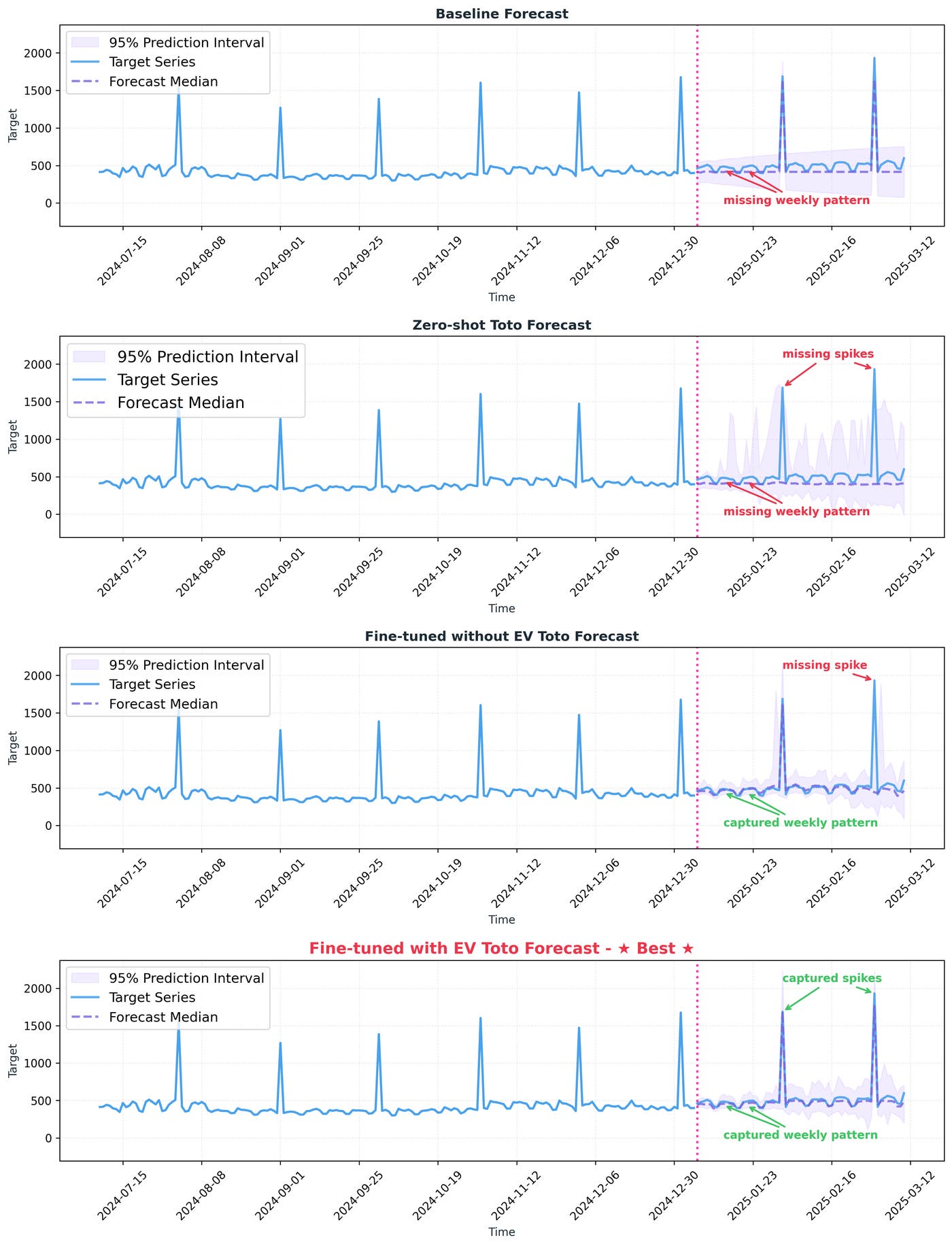
We use an example internal dataset of historical cloud spend. The task is to predict the daily cost, and we have access to a simple external covariate: a binary flag indicating if the day is the first of the month. Since billing cycles often align with the start of the month, this irregular exogenous covariate (EV) can be a significant driver of temporary spikes in spend, and including it can improve predictions.
We compare four models:
Baseline model: We use the previously deployed forecasting baseline—a tuned statistical model based on SARIMAX, with AutoARIMA for hyperparameter selection.
Toto zero-shot: We apply Toto directly to the cloud cost series without any fine-tuning or exogenous covariates.
Toto fine-tuned on the target: We fine-tune Toto on historical cost data, but still only use the target series.
Toto fine-tuned with exogenous covariates: We fine-tune Toto on a multivariate dataset that includes both historical cost and the “first day of the month” flag. At inference time, we feed Toto the future “first day of the month” flag along with the past cost history.
Visually, we can see that the zero-shot Toto forecast is unable to model the irregularly-spaced monthly seasonality; it completely fails to predict the spikes. The fine-tuned version does a better job, but still misses some of the spikes. And the version fine-tuned with the exogenous covariate (EV) comes closest to the observed values, successfully capturing the spikes at the beginning of the month, while also modeling weekly patterns that are not captured by the baseline model:
Quantitatively, we assess the forecast using a set of evaluation metrics selected by internal stakeholders: mean absolute error (MAE) and mean squared error (MSE) on the daily forecasts, and mean absolute percentage error (MAPE) on monthly roll-ups (for cloud cost data, accurately forecasting spend over the entire month is a core business objective). With no fine-tuning, zero-shot Toto fails to consistently outperform the baseline. The version of Toto fine-tuned on the target variable does manage to perform slightly better than the baseline; meanwhile, the Toto model fine-tuned with exogenous covariates (EV) shows significant improvement across all metrics.
| Metric ↓ | Baseline (SARIMAX) | Zero-shot Toto | Fine-tuned Toto without EV | Fine-tuned Toto with EV |
|---|---|---|---|---|
| MAE ↓ | 0.347 | 0.333 | 0.304 | 0.291 |
| MSE ↓ | 0.622 | 0.658 | 0.589 | 0.490 |
| MAPE (monthly) ↓ | 0.104 | 0.148 | 0.094 | 0.082 |
Table 1 shows a performance comparison of Toto variants on an internal cloud cost dataset. Metrics are aggregated from predictions over sliding windows over the test set. Best results are shown in bold; second-best results are shown in italics.
To further validate the performance of fine-tuning Toto with exogenous covariates, we tested our method on a selection of publicly available datasets. We selected a subset of 13 datasets from within the fev datatests collection—datasets with exogenous covariates, and for which there was no overlap with Toto’s pretraining data.
These benchmarks include data with exogenous covariates from various domains, including:
Energy demand forecasting, using external weather forecasting information as a predictor of expected load
Air quality forecasting, modeling pollutant concentrations conditioned on temperature and humidity measurements
Electricity price forecasting across several European markets, incorporating exogenous inputs such as generation and load forecasts
Retail demand forecasting, covering transactional orders and sales conditioned on calendar-based exogenous covariates (for example, promotions and holidays)
We see substantial improvement in average performance on standard forecasting metrics such as weighted quantile loss (WQL) and mean absolute scaled error (MASE) when going from zero-shot to fine-tuning, and an additional boost when including exogenous covariates. This is not universally the case for every individual dataset. When using Toto on your own data, it’s important to experiment on a held-out test set with different settings (zero-shot, fine-tuning, and fine-tuning with exogenous covariates) to identify the best recipe.
| Metric ↓ | Zero-shot Toto | Fine-tuned Toto without EV | Fine-tuned Toto with EV |
|---|---|---|---|
| WQL (Avg.) ↓ | 0.111 | 0.100 | 0.096 |
| WQL (Avg. Rank) ↓ | 2.284 | 1.753 | 1.499 |
| MASE (Avg.) ↓ | 0.632 | 0.574 | 0.535 |
| MASE (Avg. Rank) ↓ | 2.433 | 1.931 | 1.277 |
Table 2 shows a performance comparison of Toto variants on a selection of 13 public datasets. For each dataset, models are evaluated using sliding windows over the test split; scores are first aggregated at the dataset level and then aggregated across all datasets using a geometric mean. Best results are shown in bold; second-best results are shown in italics.
Full code for reproducing this example—including data loading, feature construction for exogenous covariates, and training scripts—is available in the Toto repository.
Let’s unpack how exogenous covariates fit into Toto’s architecture.
Toto is an autoregressive model: during training, it’s optimized to predict the next patch of the time series based on the previous patches. Concretely, we break the time series into non-overlapping patches (windows of contiguous datapoints), and for each position, the model receives a context of past patches and is trained to predict the next one. During pretraining, we shift the targets one patch forward relative to the inputs; this is analogous to how LLMs are trained to predict the next token in a sequence.
To incorporate exogenous covariates, we want the model to know the future values of those variables at each time step it’s predicting without training it to forecast those covariates themselves. Because Toto is natively multivariate (it already has the ability to model interactions between multiple variates), with slight modifications we can add known future exogenous covariates to our forecasts.
We do this in three steps:
Shift exogenous inputs forward: For the exogenous covariates, we shift the inputs forward by one patch (see Figure 2), aligning them in time with the targets, and stack them along the variate dimension. Intuitively, when Toto is asked to predict the patch at time t+1, it is given not only the history up to t, but also the values of the exogenous covariates at t+1. This ensures that, during training, the model always “knows” the exogenous covariates for every time step it is trying to predict.
Prepend a variate label token to the sequence in embedding space: Variate-wise attention in Toto is permutation invariant and does not use positional encodings. During fine-tuning, we want the model to be able to learn which variates are exogenous and how they relate to the targets. To enable this, we prepend a learnable label token to each variate sequence in embedding space, using one token for target variates and another for exogenous covariates.
Mask the loss on exogenous covariates: Since future values of the exogenous covariates are assumed to be known, we do not care about predicting them. Instead, we mask the loss for the exogenous dimensions so that Toto is only penalized for errors on the target variable(s). This allows the model to freely use the exogenous inputs as conditioning information without being forced to produce forecasts for them.
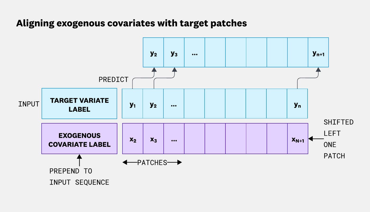
Because exogenous covariates are handled at the data and loss level, we can keep the core Toto architecture unchanged. This makes it easier to reuse existing infrastructure—model weights, inference code, and scaling strategies—while still gaining the benefits of richer side information.
If you’re working with time series that depend on known-future signals—like demand driven by holidays, cloud capacity shaped by rollouts, or energy usage influenced by weather—fine-tuning Toto with exogenous covariates is a natural next step. We’re excited to see what you’ll build with Toto’s new fine-tuning and exogenous covariates capabilities. Try fine-tuning with exogenous covariates today using the reference code and examples in the Toto repository, including the energy forecasting demo from this post.
If building models like Toto—and pushing the frontier of AI for observability—sounds exciting, check out open roles at Datadog AI Research.
此内容由惯性聚合(RSS阅读器)自动聚合整理,仅供阅读参考。 原文来自 — 版权归原作者所有。