In addition to making our FLUX.1 Kontext [dev] implementation open-source, we wanted to provide more guidance on how we chose to optimize it without compromising on quality.

In this post, you will mainly learn about TaylorSeer optimization, a method to approximate intermediate image predictions by using cached image changes (derivatives) and formulae derived from Taylor Series approximations.

Fellow optimization nerds, read on.

---

(We pulled most of our implementation info from the following paper.)

If you head to the predict function in predict.py from our FLUX.1 Kontext [dev] repo, you will find the main logic. (Highly suggest working through the repo and using this post as a guide for understanding its structure.)

Let’s break it down.

On TaylorSeer

When generating a new image with FLUX.1 Kontext, you apply a diffusion transformation across multiple timesteps — around 30 steps in a row. At each step, a stack of transformer layers predicts an update to the image you are denoising. This process can take a while.

At any given timestep, the change predicted by the model has redundancies with the predictions at previous timesteps. We could take advantage of these redundancies by caching the model’s output at certain timesteps, and reusing cached outputs at future timesteps. This “naïve caching” — where you just reuse the last feature or latent value — sometimes works OK, but can lead to blurring, loss of detail, or sometimes total distortion of the image.

You could try something slightly smarter: a linear approximation. You can estimate your next step by looking at the difference between the last two steps (i.e. a first-order finite difference) and extending the line. It’s better, but still not great. It doesn’t capture curves, acceleration, or nonlinear changes — all of which are common in diffusion models.

TaylorSeer offers a solution for this. It uses Taylor series to approximate the model’s output at a timestep using a series of cached derivatives, capturing non-linear change.

Here’s the core idea in math terms. To predict the feature at a timestep t+k in a certain layer l, we use a truncated Taylor expansion:

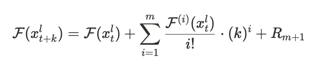
Notice the summation requires i-order derivatives of the feature function. Since we can’t compute the actual derivatives, we can use the finite difference between each i-1’th and i’th derivative. Check out the paper for the exact math, but when you perform that substitution and do a bit of simplifying, you get the following:

This is our final approximation of the feature at time step t+k.

We now have a method to speed up our diffusion process by using the above estimation for the feature at particular time steps.

We set up a TaylorSeer cache to perform this approximation when comes time:

Here, order = n_derivatives + 1. If n_derivatives = 2, for instance, then order = 3, and we cache:

• dY_current[0]: The current feature
• dY_current[1]: The first-order derivative
• dY_current[2]: The second-order derivative

The first few steps of denoise() always computes full predictions, which are used to initialize the finite differences. Later steps can be approximated.

---

Step-by-step: How TaylorSeer works in Flux Kontext

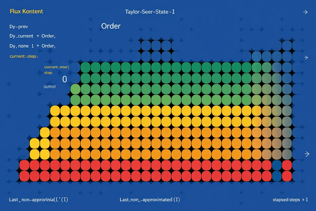
Once we’ve prepared the inputs, we decide which steps to compute and which to approximate using generate_compute_step_map():

generate_compute_step_map() follows a simple rule: always compute the first and last few steps, since that’s where the model makes the biggest changes. In the middle steps, we compute every other step for “go fast” mode, or every third step for “go really fast.” An adaptive approach like First Block Cache, which checks how much the first transformer block output changes, could be smart to ascertain which steps to skip, but this hard-coded strategy works well.

Two paths: compute or approximate

In the denoising loop:

Let’s break down each path.

---

Path 1: Full computation

We run the model normally and update our stored finite differences (derivatives):

This is a recursive view of computing higher-order finite differences from the lower-order ones. The m+1’th order derivative comes from the difference of the m’th order derivative values over the time that passed.

These differences approximate how the feature values evolve over time.

---

Path 2: Approximate using Taylor series

If we decide to skip a step (based on compute_step_map), we use the cached differences to estimate the next feature update (our approximation from equation 2):

The time it takes to compute this approximation is nearly instantaneous compared to the time it takes to run the full model for a single denoising step.

---

Update the latent

At every step, whether we computed or approximated, we apply the predicted delta to the image latent:

This keeps the image transformation evolving across timesteps.

---

After the denoise loop, we return our final image!

Summary

Instead of evaluating the model at every single timestep, we:

1. Cache past predictions and their finite differences.
2. Use Taylor series to approximate the model’s output at skipped steps.
3. Reduce model calls from 30 to maybe 10–15, depending on speed settings.
4. Maintain quality, especially at the start and end of generation, where accuracy matters most.

TaylorSeer gives us a principled, flexible way to forecast intermediate steps in image generation using feature dynamics. It’s faster than running every step and smarter than linear extrapolation.

You can find this all in denoise() and taylor_utils.py in our FLUX.1 Kontext repo.

Hammer away at the repo, and let us know what you discover!