Differentiating through optimization is a fundamental problem in hyperparameter optimization, dataset distillation, meta-learning and optimization as a layer, to name a few. In this blog post we'll look into one of the main approaches to differentiate through optimization: unrolled differentiation. With the help of polynomials, we'll be able to derive tight convergence rates and explain some of its most puzzling behavior.

Understanding Implicit Functions in Machine Learning

Implicit functions are functions that lack a closed form expression and instead are defined as the solution of an optimization problem or as the solution of a set of equations.

A classic example of implicit function is the model parameters of a machine learning model when viewed as a function of the regularization parameter. For example, let $\ell(\xx, \boldsymbol{a_i}, b_i)$ denote the loss incurred with model parameters $\xx$ on the sample $(\boldsymbol{a}_i, b_i)$. Then the model parameters $\xx_\star(\theta)$ are the minimizers of the empirical risk plus a regularization term: \begin{align} \xx_\star(\theta) \defas \argmin_{\zz \in \RR^d} \frac{1}{n}\sum_{i=1}^n \ell(\zz,\boldsymbol{a_i}, b_i) + \theta \| \zz \|^2 \,. \end{align} Except for simple problems like ordinary least squares regression, the function $\xx_\star(\theta)$ lacks a closed form expression and is instead represented implicitly as the optimization problem above.

Dataset distillation, is a distinct problem that aims to learn a few synthetic images for training a model with the highest possible test set accuracy. 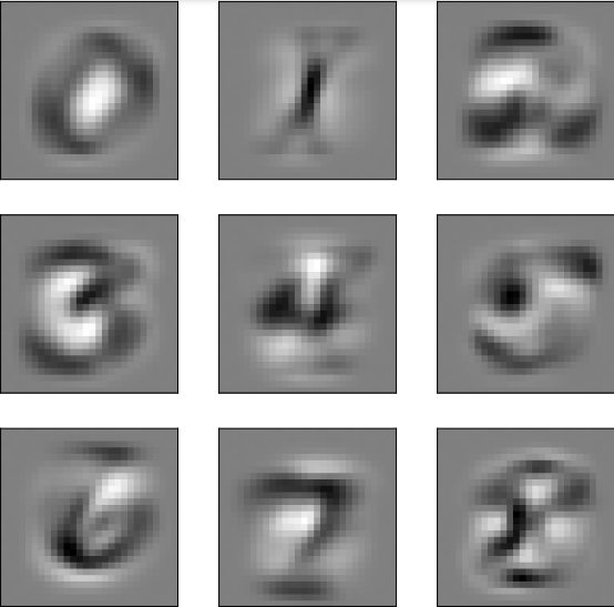First 9 digits estimated through dataset distillation. A logistic regression model trained exclusively on the above achieves 80% generalization accuracy on MNIST. Example from the JAXopt notebook gallery.

There are many other applications of implicit functions in machine learning, such as learned data augmentation (the data augmentation function is parameterized by $\ttheta$),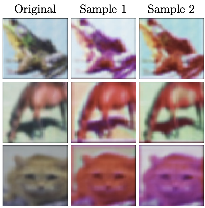
Learned data augmentation. The original image is on the left, followed by two augmented samples. Figure source: (Lorraine et al. 2020) architecture search ($\ttheta$ describes the network architecture), meta-learning ($\ttheta$ is a regularization bias), federated learning, and optimization as a layer (where $\ttheta$ are the activations of the previous layer).

The main challenge with implicit functions is computing the Jacobian $\partial \xx(\ttheta)$, which is essential for gradient-based optimization. There are two main approaches. The most classical one is based on the implicit function theorem and allows to recover the desired Jacobian as the solution to a linear system.

The other approach for computing the Jacobian $\partial \xx(\ttheta)$, which is the one we'll be considering today, is based on combining automatic differentiation with an optimization algorithm. It was initially developed under the name of piggyback differentiation and has been rediscovered many times under different names such as differentiating through optimization and unrolled differentiation, For convenience, I'll just call it unrolling.

With the help of polynomials, we'll analyze the convergence of unrolling, and unravel some of its mysteries and puzzling behavior. This blog post is based upon our paper (Scieur et al. 2022). See also Section 5 below for a more complete set of references and related works.

Unrolled Differentiation

In this section we'll describe more precisely the method of unrolled differentiation.

Throughout the rest of this post we'll denote by $f(\cdot, \ttheta)$ the cost that defines the implicit function $\xx_\star(\ttheta)$: \begin{equation} \xx_\star(\ttheta) = \argmin_{\zz \in \RR^d} f(\zz, \ttheta)\,. \end{equation} For simplicity, we'll assume that the minimizer of $f(\cdot, \ttheta)$ is unique, as otherwise the implicit function would be set-valued.This assumption is not violated for example on over-parameterized models and non-convex objectives. The study of these functions opens some fascinating questions, as explored in the next reference. Unrolling is a method to approximate the Jacobian $\partial \xx_\star(\ttheta)$.

\begin{equation}\label{eq:opt} \begin{aligned} &\qquad \textbf{Goal:} \text{ approximate } \partial \xx_\star(\ttheta)\,, \\ &\text{where } \xx_\star(\ttheta) = \argmin_{\zz \in \RR^d} f(\zz, \ttheta) \,. \end{aligned} \end{equation}

Unrolling assumes access to an optimization method that generates a sequence $\xx_1(\ttheta), \xx_2(\ttheta), \xx_3(\ttheta), \ldots$ converging to $\xx_\star(\ttheta)$. Let $F_t$ denote the update that generates the next iterate $\xx_{t}$ from the previous ones : \begin{equation} \xx_t(\ttheta) = F_t(\xx_{t-1}(\ttheta), \ldots, \xx_0(\ttheta), \ttheta)\,. \end{equation} This formulation is versatile, accommodating most optimization methods. For example, for gradient descent we would have $F_t(\xx_{t-1}, \ldots, \xx_0, \ttheta) = \xx_{t-1}(\ttheta) - \gamma \partial_1 f(\xx_{t-1}, \ttheta)$. We'll use the notation $\partial_i$ to denote differentiation with respect to the $i$-th argument of a function. We'll drop the subindex for functions of a single argument.

The key idea behind unrolled differentiation is that differentiating both sides of the above recurrence and using the chain rule gives a recurrence for the Jacobian: \begin{equation}\label{eq:jacobian_recurrence} \partial \xx_t(\ttheta) = \sum_i \partial_i F(\xx_{t-1}, \ldots, \xx_0, \ttheta) \partial \xx_i \end{equation}

The use of $\partial \xx_t(\ttheta)$ as an approximation to the true Jacobian $\partial \xx_\star(\ttheta)$ is justified by the fact that under smoothness assumptions, the limit and derivative are exchangeable,Can I exchange limit and differentiation for a sequence of smooth functions?Math stackexchange so if $\xx_t$ converges to $\xx_\star$, then $\partial \xx_t$ converges to $\partial \xx_\star$. For notational simplicity, we'll omit sometimes the dependence on $\ttheta$ in the rest of the post, so that $\xx_t$ denotes $\xx_t(\ttheta)$ and $\partial \xx_t$ denotes $\partial \xx_t(\ttheta)$.

Expressions for other solvers can be computed in a similar way. Furthermore, one usually doesn't need to manually derive the recurrence \eqref{eq:jacobian_recurrence}, as automatic differentiation software (such as JAX, PyTorch, Tensorflow, etc.) can take care of that.The associated Colab contains several JAX examples.

A Quadratic Model for Unrolling

In the rest of the blog post we'll assume that the objective function $f$ is a quadratic function in its first argument of the form \begin{equation} % \vphantom{\sum^i_n} f(\xx, \ttheta) \defas \tfrac{1}{2} \xx^\top \HH(\ttheta)\, \xx + \bb(\ttheta)^\top \xx\,, \end{equation} where $\ell \II \preceq \HH(\ttheta) \preceq L\II$ for some scalars $\ell$ and $L$. This model includes problems such as ridge regression with $\HH(\ttheta) = \HH + \theta I$

The polynomial formalism is based on the following observation: for a fixed value of $\ttheta$, the error sequence $\xx_0 - \xx_\star, \xx_1 - \xx_\star, \ldots$ can be expressed compactly as \begin{equation}\label{eq:residual_polynomial} \xx_t - \xx_\star = {\color{colorresidual}P_t(\HH(\ttheta))}(\xx_0 - \xx_\star)\,, \end{equation} where ${\color{colorresidual}P_t(\HH(\ttheta))}$ is a $t$-th degree (matrix-valued) polynomial in $\HH(\ttheta)$. We'll refer to this polynomial ${\color{colorresidual}P_t}$ as the residual polynomial. Thanks to the polynomial formalism we can leverage the rich theory of polynomials to analyze the convergence of optimization methods (and now urolling methods, too).

How Fast is Unrolling?

Deriving both sides of the above identity \eqref{eq:residual_polynomial} with respect to $\ttheta$, we obtain a new identity, this time where the left hand side is the Jacobian error $\partial \xx_t(\ttheta) - \partial \xx_\star(\ttheta)$ and the right-hand side contains both the polynomial ${\color{colorresidual}P_t}$ and its derivative ${\color{teal}P_t'}$. This identity will be the key to our convergence-rate analysis, as the Jacobian error is precisely the quantity we wish to bound.

The following theorem provides a convenient formula for the Jacobian error, which we'll use to derive convergence rates for unrolling methods. It makes a technical assumptions that $\HH(\theta)$ commutes with its Jacobian (which is verified for example in the case of ridge regression, where $\partial \HH(\ttheta)$ is the identity).

Let $\xx_t(\ttheta)$ be the $t^{\text{th}}$ iterate of a first-order method associated to the residual polynomial $P_t$. Assume furthermore that the $\HH(\theta)$ commutes with its Jacobian, that is, $\partial \HH(\ttheta)_i \HH(\ttheta) = \HH(\ttheta)\partial \HH(\ttheta)_i~\text{ for } 1 \leq i \leq k\,.$ . Then the Jacobian error can be written as \begin{equation} \begin{aligned} &\partial \xx_t(\ttheta) - \partial \xx_\star(\ttheta)\\ &\quad= \big({\color{colorresidual}P_t(\HH(\ttheta))} - {\color{teal}P_t'(\HH(\ttheta))}\HH(\ttheta)\big) (\partial \xx_0(\ttheta)-\partial \xx_\star(\ttheta)) \nonumber\\ &\qquad+ {\color{teal}P_t'(\HH(\ttheta))} \partial_\ttheta\nabla f(\xx_0(\ttheta), \ttheta)\,. \end{aligned}\label{eq:distance_to_optimum} \end{equation}

See Appendix C of (Scieur et al., 2022).

The key difference between the formula for the Jacobian suboptimality \eqref{eq:distance_to_optimum} and that of the iterates suboptimality \eqref{eq:residual_polynomial} is that the first one involves not only the residual polynomial ${\color{colorresidual}P_t}$ but also its derivative ${\color{teal}P_t'}$.

This has important consequences. For example, while the residual polynomial might be monotonically decreasing in $t$, its derivative might not be. This is in fact the case for gradient descent, whose residual polynomial ${\color{colorresidual}P_t}(\lambda) = (1 - \gamma \lambda)^{-t}$ is decreasing in $t$, but whose derivative ${\color{teal}P_t'}(\lambda) = \gamma t (1 - \gamma \lambda)^{-t-1}$ is not.

In fact, we can use the above theorem to derive tight convergence rate for many methods by plugging in the method's residual polynomial. For example, for gradient decent we can derive the following convergence rate.

Under the same assumptions as the previous theorem and with $G \defas \| \partial_\ttheta\nabla f(\xx_0(\ttheta), \ttheta)\|_F.$, let $\xx_t(\ttheta)$ be the $t^{\text{th}}$ iterate of gradient descent scheme with step size $h>0$. Then, \begin{equation*} \|\partial \xx_t(\ttheta) - \partial \xx_\star(\ttheta)\|_F \leq \max_{\lambda \in[\ell, L]} \Big| {\underbrace{\left( 1-h\lambda \right)^{t-1}}_{\text{exponential decrease}}}\big\{ {\underbrace{(1+(t-1)h\lambda)}_{\text{linear increase}}} \|\partial \xx_0(\ttheta)-\partial \xx_\star(\ttheta)\|_F + {\vphantom{\sum_i}h t} G \big\}\,\Big|. \end{equation*}

Unlike for the iterate suboptimality (whose rate is $\| \xx_t(\ttheta) - \xx_\star(\ttheta)\| \leq \max_{\lambda \in[\ell, L]} \left( 1-h\lambda \right)^{t-1} \|\xx_0(\ttheta)-\xx_\star(\ttheta)\|$), the Jacobian suboptimality rate is not monotonic in $t$. In fact, it has an initial increasing phase during which the linear increase term ${(1+(t-1)h\lambda)}$ dominates, followed by a decreasing phase during which the exponential decrease term ${(1-h\lambda)^{t-1}}$ dominates.

This can be seen in the following plot, where we plot side-by-side the suboptimality in both cases. In the right side we show the optimization error, which are the iterates' error norm $\|\xx_t - \xx_\star\|$ where $\xx_t$ is the result fo doing $t$ steps of gradient descent and $\xx_\star$ is the minimizer of the above over $\xx$, and for a fixed $\theta$. The right hand side shows instead the unrolling error, which is the norm of the difference between the Jacobian estimated after t steps of gradient descent $\partial \xx_t$ and the true Jacobian $\partial \xx_\star$.

The Jacobian suboptimality shows an initial increase in suboptimality during early iterations

Furthermore, this initial increase in suboptimality becomes longer and more pronounced as the step-size increases. This shows an inherent trade-off in the step-size selection of unrolling: a large step-size will lead to a faster asymptotic convergence rate, but will also lead to a longer initial phase of increasing suboptimality. A small step-size on the other hand will lead to a shorter initial phase of increasing suboptimality, but will also lead to a slower asymptotic convergence rate. We called this phenomenon the curse of unrolling.

The curse of unrolling is not limited to gradient descent. It is a general phenomenon that steps from the fact that the Jacobian suboptimality contains a factor of the derivative of the residual polynomial, which can be arbitrarily large for some methods. For example, we saw above that for gradient descent, the rate of unrolling has an extra factor of $t$ that makes it initially increase. Similarly, the rate of unrolling for Chebyshev's method (which has optimal worst-case rate for the optimization error) has an extra factor of $t^2$ in the rate, which makes it initially increase even faster.

Under the same assumptions as the previous theorem, let $\xi \defas (1-\sqrt{\kappa})/(1+\sqrt{\kappa})$ with $\kappa \defas \ell/L$, and $\xx_t(\ttheta)$ denote the $t^{\text{th}}$ iterate of the Chebyshev method. Then, we have the following convergence rate \begin{align*} \|\partial \xx_t(\ttheta) - \partial \xx_\star(\ttheta)\|_F & \leq {\underbrace{\left(\tfrac{2}{\xi^t+\xi^{-t}}\right)}_{\text{exponential decrease}}} \Bigg\{{\underbrace{\vphantom{\left(\tfrac{1-\kappa}{1+\kappa}\right)^{t-1}}\left| \tfrac{2t^2}{1-\kappa}-1 \right|}_{\vphantom{p}\text{quadratic increase}}}\|\partial \xx_0(\ttheta) - \partial \xx_\star(\ttheta)\|_F + {\vphantom{\left(\tfrac{1-\kappa}{1+\kappa}\right)^{t-1}} \frac{2t^2}{L-\ell}} G \Bigg\}\,. \end{align*} In short, the rate of the Chebyshev algorithm for unrolling is $O( t^2\xi^t)$.

To know more

While in this blog post we choose the polynomial formalism to analyze unrolling, this is not the only option. There has been some recent work on analyzing unrolling methods beyond quadratic problems, see for example (Grazzi et al. 2020) and (Ablin et al. 2020). (Brauer et al., 2022) Although these works are more widely applicable than the quadratic setting of this post, the rates are looser and the analysis more involved.

Another advantage of the polynomial formalism that we haven't exploited in this post but we'll do in future ones is that it allows to derive optimal algorithms in a constructive way, which is not possible with the more general analysis.

Shortly before I released this blog post, Felix Köhler made an excellent video on the curse of unrolling. I highly recommend checking it out for a more hands-on tutorial!

Citing

If you find this blog post useful, please consider citing its accompanying paper as

The Curse of Unrolling: Rate of Differentiating Through Optimization, Scieur, Damien, Quentin Bertrand, Gauthier Gidel, and Fabian Pedregosa.. Advances in Neural Information Processing Systems 35 (NeurIPS 2022), 2022

Bibtex entry:

    
      @inproceedings{scieur2022curse,
        title={The Curse of Unrolling: Rate of Differentiating Through Optimization},
        author={Scieur, Damien and Bertrand, Quentin and Gidel, Gauthier and Pedregosa, Fabian},
        booktitle={Advances in Neural Information Processing Systems 35},
        year={2022}
      }
    
    

References