Suppose some given data points each belong to one of two classes, and the goal is to decide which class a new data point will be in. In the case of support vector machines, a data point is viewed as a p-dimensional vector (2-dimensional in this example), and we want to know whether we can separate such points with a p -1-dimensional hyperplane (a line in our case). There are many hyperplanes that might classify the data. One reasonable choice as the best hyperplane is the one that represents the largest separation, or margin, between the two classes. So we choose the hyperplane so that the distance from it to the nearest data point on each side is maximized. If such a hyperplane exists, it is known as the maximum-margin hyperplane and the linear classifier it defines is known as a maximum margin classifier. Using the new svm module in scikits.learn, you can easily plot the maximum margin hyperplane. If clf is an instance of svm.SVC(), the coefficients in the decision function are stored in clf.coef_ , and the independent term in clf.rho_ . The complete source code is: [cc lang="python"] import numpy as np import pylab as pl from scikits.learn import svm # we create 40 separable points np.random.seed(0) X = np.r_[np.random.randn(20, 2) - [2,2], np.random.randn(20, 2) + [2, 2]] Y = [0]*20 + [1]*20 # fit the model clf = svm.SVC(kernel='linear') clf.fit(X, Y) # get the separating hyperplane w = np.dot(clf.coef_[0], clf.support_) a = -w[0]/w[1] xx = np.linspace(-5, 5) yy = a*xx + (clf.rho_[0])/w[1] # plot the paralels to the separating hyperplane that pass through the # support vectors b = clf.support_[0] yy_down = a*xx + (b[1] - a*b[0]) b = clf.support_[-1] yy_up = a*xx + (b[1] - a*b[0]) # plot the line, the points, and the nearest vectors to the plane pl.set_cmap(pl.cm.Paired) pl.plot(xx, yy, 'k-') pl.plot(xx, yy_down, 'k--') pl.plot(xx, yy_up, 'k--') pl.scatter(X[:,0], X[:,1], c=Y) pl.scatter(clf.support_[:,0], clf.support_[:,1], marker='+') pl.axis('tight') pl.show() [/cc] And the result is

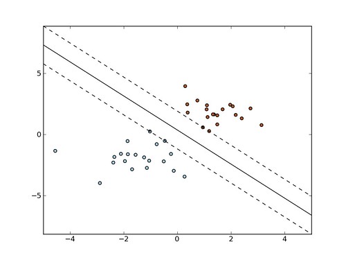
where the vectors that are closest to the separating line are highlighted with a small '+'. Up-to date code of this can be found in directory examples/ of scikits.learn