










While the most common accelerated methods like Polyak and Nesterov incorporate a momentum term, a little known fact is that simple gradient descent –no momentum– can achieve the same rate through only a well-chosen sequence of step-sizes. In this post we'll derive this method and through simulations discuss its practical limitations.
Residual Polynomials and the Chebyshev iterative method
As in previous installments if this series of blog posts, our motivating problem is that of finding a real-valued vector $\xx^\star$ that minimizes the quadratic function \begin{equation}\label{eq:opt} f(\xx) \defas \frac{1}{2}\xx^\top \HH \xx + \bb^\top \xx~, \end{equation} where $\HH$ is a $d\times d$ positive definite matrix with bounded eigenvalues in the interval $[\lmin, L]$.
I described in the first part of this series a connection between optimization methods and polynomials that allows to cast complexity analysis of optimization methods as a problem of bounding polynomials and which I'll be using extensively here. Through this connection, each optimization method determines a sequence of polynomials that determine the convergence of the method. More precisely, after $t$ iterations, we can associate to every optimization method a polynomial $P_t(\lambda) = a_t \lambda^t + \cdots + 1$ of degree $t$ and $P_t(0) = 1$ such that the error at iteration $t$ is given in terms of this polynomial as$P_t(\HH)$ represents the output of evaluating the originally real-valued polynomial $P_t(\cdot)$ at the matrix $\HH$. I'm being a bit liberal with notation here, as $P_t$ represents both the real-valued and matrix-valued polynomial depending on the input. \begin{equation} \xx_t - \xx^\star = P_t(\HH)(\xx_0 - \xx^\star)\,. \end{equation}
As we saw in the first part of this series, there's a very illustrious polynomial that minimizes the worst-case convergence rate $\max_{\lambda \in [\lmin, L]}|P_t(\lambda)|$: the scaled and shifted Chebyshev polynomial \begin{equation} P^\text{Cheb}_t(\lambda) = \frac{T_t(\sigma(\lambda))}{T_t(\sigma(0))}\,, \end{equation} where $T_t$ is the $t$-th degree Chebyshev polynomial and $\sigma$ is the link function $\sigma(\lambda) = \frac{L+\lmin}{L-\lmin} - \frac{2}{L - \lmin}\lambda$.
Back then we reverse-engineered an optimization method that has as associated residual polynomial the above shifted Chebyshev polynomial. It turns out that this is not the only way to construct a method that has $P^\text{Cheb}_t$ as its residual polynomial. There are many other ways to do this, and at least one of them doesn't require a momentum term.
Young's method
Consider the gradient descent method with variable step-size. This method has a recurrence of the form \begin{equation} \xx_{t+1} = \xx_t - {\color{colorstepsize} h_t} \nabla f(\xx_t)\,. \end{equation} with one scalar parameter per iteration: the step-size ${\color{colorstepsize} h_t}$.
Subtracting $\xx^\star$ from both sides of the above equation and using the fact that for quadratic objectives $\nabla f(\xx) = \HH \xx$ we have \begin{align} \xx_{t+1} - \xx^\star &= (\II - {\color{colorstepsize}h_t} \HH) (\xx_t - \xx^\star)\\ &= (\II - {\color{colorstepsize}h_t}\HH)(\II - {\color{colorstepsize}h_{t-1}}\HH) (\xx_{t-1} - \xx^\star)\\ &= \cdots \\ &= (\II - {\color{colorstepsize}h_t}\HH)(\II - {\color{colorstepsize}h_{t-1}}\HH)\cdots (\II - {\color{colorstepsize}h_0}) (\xx_0 - \xx^\star)\,, \end{align} and so the residual polynomial associated with this method is \begin{align} P^{\text{GD}}_t(\lambda) = (1 - {\color{colorstepsize} h_t} \lambda)(1 - {\color{colorstepsize} h_{t-1}} \lambda) \cdots (1 - {\color{colorstepsize} h_0} \lambda)\,. \end{align}
Since the residual polynomial determines the convergence of a method, a simple way to ensure that the variable step-size gradient descent method has the same convergence as the Chebyshev iterative method is to find the parameters –in this case the step-size– that make $P^{\text{GD}}_t$ equal to the Chebyshev residual polynomial.
David Young
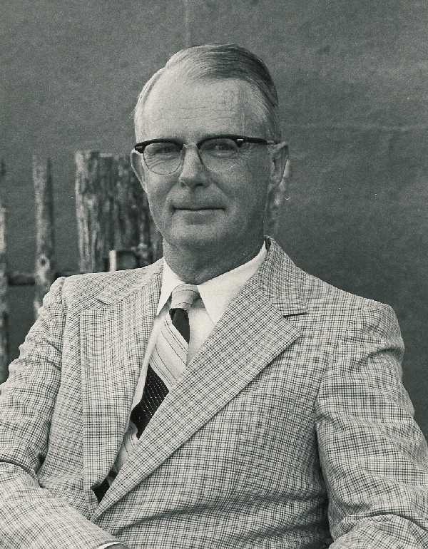
David Young (1923-2008) was an American mathematician and computer scientist. He is known for some of the most successful linear algebra methods such as successive over-relaxation and symmetric successive over-relaxation. devised in 1953 an elegant approach to set these parameters. The main motivation of this algorithm at the time was to save memory by avoiding the momentum term. Although computer capabilities have expanded greatly since then, memory is often still the bottleneck (Anil et al. 2019). His method uses the fact that the $P^{\text{GD}}_t$ polynomial above is already in factored form and its roots are
\begin{equation}\label{eq:roots_gd}
\frac{1}{{\color{colorstepsize} h_0}}, \frac{1}{{\color{colorstepsize} h_1}}, \ldots, \frac{1}{{\color{colorstepsize}
h_t}}\,.
\end{equation}
Young's key insight is that to construct the same residual polynomial it's sufficient that the roots match, as the scale is anyway fixed by the residual polynomial constraint $P_t(0) = 1$. This approach is practical because the roots of Chebyshev polynomials are easy to derive using known identities between these polynomials and trigonometric functions.
The roots of the $t$-th degree Chebyshev residual polynomial $P^\text{Cheb}_t$ are given by \begin{equation}\label{eq:chebyshev_roots} \lambda_i = {\textstyle \frac{1}{2}(L + \lmin) + \frac{1}{2}(L - \lmin)\cos\left(\frac{\pi(i+1/2)}{t}\right)}\,, \end{equation} for $i=0, \ldots, t-1$.
The Chebyshev polynomial $T_t$ can be characterized as the polynomial of degree $t$ that verifies \begin{equation} T_t(\cos(\theta)) = \cos(t \theta)\,. \end{equation} Since $\cos((i + 1/2) \pi) = 0$ for any integer $i$, the right-hand size is zero for $\theta = (i+1/2)\pi/t$, and so the roots of the Chebyshev polynomialThese roots are sometimes called Chebyshev nodes because they are used as nodes in polynomial interpolation. $T_t$ are given by \begin{equation} \xi_i = {\textstyle \cos\left(\frac{\pi(i+1/2)}{t}\right),}~ i=0,\ldots,t-1\,. \end{equation}
From the roots of the Chebyshev polynomials, we can find the roots of the shifted Chebyshev polynomial $P^\text{Cheb}_t$ by solving $\sigma(\lambda_i) = \xi_i$ for $\lambda_i$, which gives the desired value $\lambda_i$ above.
These roots also have a nice trigonometric interpretation, as they correspond to the projection onto the $x$-axis of $t$ equally spaced points on the semicircle between $\lmin$ and $L$.

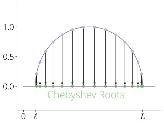
Coming back to Young's method, if we set the step-size parameters as \begin{equation} {\color{colorstepsize} h_i} = \frac{1}{\lambda_i}\,, i = 0, \ldots, t-1\,, \end{equation} where $\lambda_i$ are Chebyshev roots in the previous Theorem, the residual polynomial for this method and the Chebyshev residual polynomial at iteration $t$ are identical. Furthermore, this is true irrespective of the order in which the step-sizes are taken. For now let's take the steps in increasing order and see what happens. We'll reconsider this reckless decision later on.
Putting it all together, we can finally write Young's method:
Young's Method
Input: starting guess $\xx_0$ and $t_{\max}$.
For $t=0, \ldots, t_{\max}$ compute
\begin{align*}
&\quad{\color{colorstepsize}
h_t} = 2\big({(L + \lmin) + (L -
\lmin)\cos({(t - \tfrac{1}{2})}\tfrac{\pi}{t_{\max}})}\big)^{-1}\\
&\quad\xx_{t+1} = \xx_t - {\color{colorstepsize}
h_t}\nabla f(\xx_t)
\end{align*}
An empirical comparison of this method vs gradient descent and the Chebyshev iterative method on synthetic data confirms that this method achieves the same last-iterate convergence rate.
Young's method has the same last-iterate convergence rate than the Chebyshev iterative method on quadratic problems. The suboptimality of previous iterates is substantially different and depends on the step-size ordering.
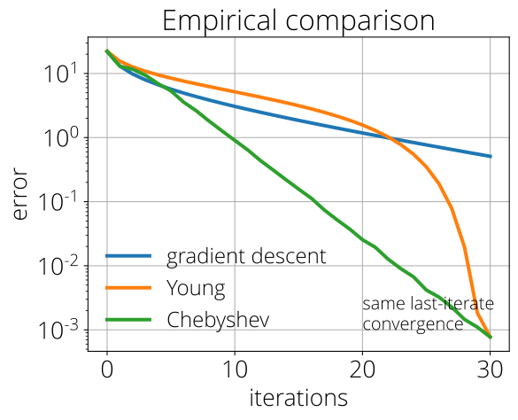
As is clear from the plot above, in Young's method only the last iterate has a rate of convergence that matches that of the Chebyshev method. This is because its residual polynomial coincides with the shifted Chebyshev polynomial $P^\text{Cheb}_t$ only at the last iterate. In contrast, for the Chebyshev method, the residual polynomial at each iterate is the residual Chebyshev polynomial $P^\text{Cheb}_t$, making it optimal at every iteration, and not only at the last iterate.Another way to say this is that Chebyshev is an anytime algorithm, while Young's method isn't.
A practical drawback is that one needs to know the number of iterations in advance. However, in practice it's more convenient to set a tolerance and not a maximum number of iterations.
Beware of Numerical Errors!
As was already noted by Young, this method is unfortunately very numerically unstable. As the number of iterations $t_{\max} $ grows, the maximum step-size converges to $1/\lmin$, which can become problematic when $\lmin$ is small as then small errors in the computation of $\lmin$ get amplified.
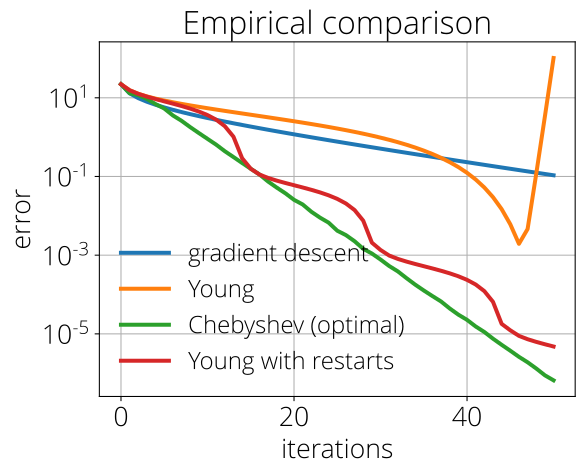
For example, in the same setting as the previous figure, I'm increasing the number of iterations from 30 to 50, which is sufficient to see a divergence of the error in the last few iterates.
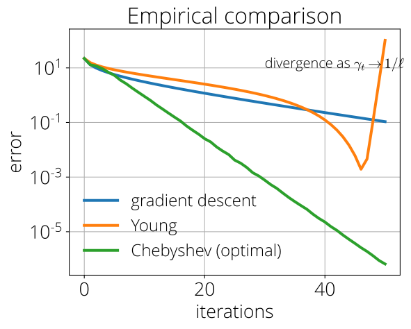
A simple workaround is to avoid the step-size getting too close to $1/\lmin$ is to limit the number of maximum iterations $t_{\max}$ to something small, and then start over once we visited the $t_{\max}$ step-sizes. I call this method the "Young's method with restarts".
Young's Method with Restarts
Input: starting guess $\xx_0$ and restarting length $t_{\text{cycle}}$.
For $t=0, 1, \ldots$ compute
\begin{align*}
&\quad k = t\bmod t_{\text{cycle}} \\
&\quad{\color{colorstepsize}
h_t} = 2\big({(L + \lmin) + (L -
\lmin)\cos({( k- \tfrac{1}{2})}\tfrac{\pi}{t_{\text{cycle}}})}\big)^{-1}\\
&\quad\xx_{t+1} = \xx_t - {\color{colorstepsize}
h_t}\nabla f(\xx_t)
\end{align*}
Although this method is no longer optimal,Or, to be more precise, it is only optimal when stopped after $t_{\text{cycle}}$ iterations, in which case it coincides with the standard Young method. it avoids some of the numerical issues of the standard method. See below a comparison on the same problem as above when I take $t_{\text{cycle}}$ to be 15:
A connection with cosine annealing and other recent work
Theres all sorts of connections still to be made between variable step-size methods and acceleration.
An obvious question is whether any of this extends to the stochastic setting. Although I don't have an answer for this, there are some similarities between this method and the recently proposed and wildly successfulAs of August 2020, the paper counts more than 1000 citations. See also my recent blog post on cyclical step-sizes. cosine annealing step-size \begin{align*} h_i &= h_{\min} + \tfrac{1}{2}(h_{\max} - h_{\min})(1 + \cos(\frac{i}{t_{\max}}\pi))\\ &= \tfrac{1}{2}(h_{\min} + h_{\max}) + \tfrac{1}{2}(h_{\max} - h_{\min}) \cos(\frac{i}{t_{\max}}\pi) \end{align*} which is equal to the inverse of the Chebyshev roots \eqref{eq:chebyshev_roots}, modulo the very minor modification $i+1/2 \to i$.
After writing this blog post, I became aware of this recent paper by Naman Agarwal, Surbhi Goel and Cyril Zhang that proposes a fractal ordering of the step-sizes. They show that this ordering is more robust, and also provide robustness analysis, experimental validation and links with the Soviet literature that I was unaware of. Definitely worth checking out!
Citing
If you find this blog post useful, please consider citing it as:
Acceleration without Momentum, Fabian Pedregosa, 2021
Bibtex entry:
    @misc{pedregosa2021nomomentum,
      title={Acceleration without Momentum},
      author={Pedregosa, Fabian},
      howpublished = {\url{http://fa.bianp.net/blog/2021/no-momentum/}},
      year={2021}
    }
Thanks
This blog post grew out of numerous discussions with collaborators Nicolas Le Roux and Damien Scieur. A note of gratitude is due also to Konstantin Mischenko, for constructive comments and for suggesting the name "Young method with restarts".