Besides performing a line-by-line analysis of memory consumption, memory_profiler exposes some functions that allow to retrieve the memory consumption of a function in real-time, allowing e.g. to visualize the memory consumption of a given function over time.

The function to be used is memory_usage. The first argument specifies what code is to be monitored. This can represent either an external process or a Python function. In the case of an external process the first argument is an integer representing its process identifier (PID). In the case of a Python function, we need pass the function and its arguments to memory_usage. We do this by passing the tuple (f, args, kw) that specifies the function, its position arguments as a tuple and its keyword arguments as a dictionary, respectively. This will be then executed by memory_usage as f(*args, **kw).

Let's see this with an example. Take as function NumPy's pseudo-inverse function. Thus f = numpy.linalg.pinv and f takes one positional argument (the matrix to be inverted) so args = (a,) where a is the matrix to be inverted. Note that args must be a tuple consisting of the different arguments, thus the parenthesis around a. The third item is a dictionary kw specifying the keyword arguments. Here kw is optional and is omitted.

>>> from memory_profiler import memory_usage
>>> import numpy as np
# create a random matrix
>>> a = np.random.randn(500, 500)
>>> mem_usage = memory_usage((np.linalg.pinv, (a,)), interval=.01)
>>> print(mem_usage)
[57.02734375, 55.0234375, 57.078125, ...]

This has given me a list specifying at different time intervals (t0, t0 + .01, t0 + .02, ...) at which the measurements where taken. Now I can use that to for example plot the memory consumption as a function of time:

>>> import pylab as pl
>>> pl.plot(np.arange(len(mem_usage)) * .01, mem_usage, label='linalg.pinv')
>>> pl.xlabel('Time (in seconds)')
>>> pl.ylabel('Memory consumption (in MB)')
>>> pl.show()

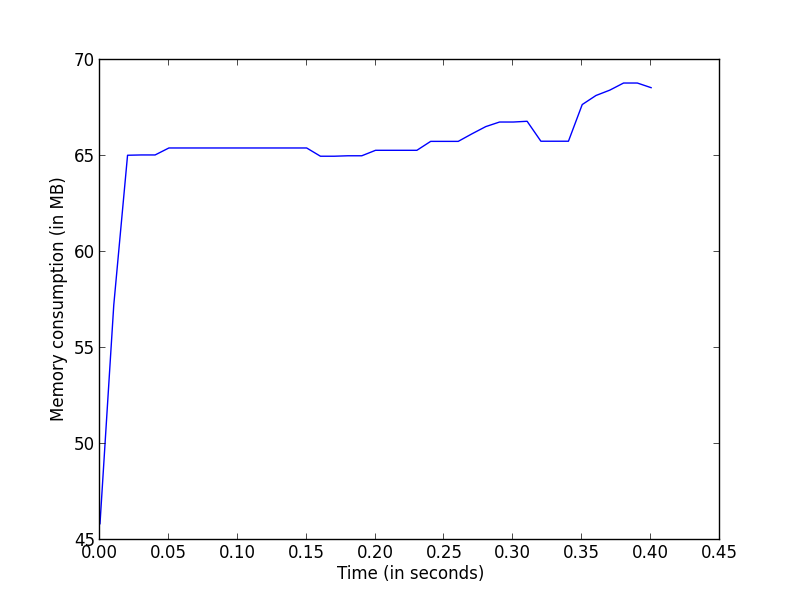
This will give the memory usage of a single function across time, which might be interesting for example to detect temporaries that would be created during the execution.

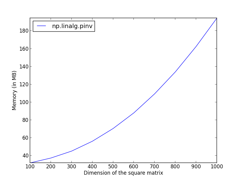
Another use case for memory_usage would be to see how memory behaves as input data gets bigger. In this case we are interested in memory as a function of the input data. One obvious way we can do this is by calling the same function each time with a different input and take as memory consumption the maximum consumption over time. This way we will have a memory usage for each input.

>>> for i in range(1, 5):
...    A = np.random.randn(100 * i, 100 * i)
...    mem_usage = memory_usage((np.linalg.pinv, (A,)))
...    print max(mem_usage)

29.22
30.10
40.66
53.96

It is now possible to plot these results as a function of the dimensions.

import numpy as np
import pylab as pl
from memory_profiler import memory_usage

dims = np.linspace(100, 1000, 10)
pinv_mem = np.zeros(dims.size)

for i_dim, k in enumerate(dims):
    x = np.random.randn(k, k)
    tmp = memory_usage((np.linalg.pinv, (x,)), interval=.01)
    pinv_mem[i_dim] = np.max(tmp)

pl.plot(dims, pinv_mem, label='np.linalg.pinv')
pl.ylabel('Memory (in MB)')
pl.xlabel('Dimension of the square matrix')
pl.legend(loc='upper left')
pl.axis('tight')
pl.show()