In this post I compar several implementations of Logistic Regression. The task was to implement a Logistic Regression model using standard optimization tools from scipy.optimize and compare them against state of the art implementations such as LIBLINEAR.

In this blog post I'll write down all the implementation details of this model, in the hope that not only the conclusions but also the process would be useful for future comparisons and benchmarks.

Function evaluation

We consider the case in which the decision function is an affine function, i.e., $f(x) = \langle x, w \rangle + c$ where $w$ and $c$ are parameters to estimate. The loss function for the $\ell_2$-regularized logistic regression, i.e. the function to be minimized is

$$ \mathcal{L}(w, \lambda, X, y) = - \frac{1}{n}\sum_{i=1}^n \log(\phi(y_i (\langle X_i, w \rangle + c))) + \frac{\lambda}{2} w^T w $$

where $\phi(t) = 1. / (1 + \exp(-t))$ is the logistic function, $\lambda w^T w$ is the regularization term and $X, y$ is the input data, with $X \in \mathbb{R}^{n \times p}$ and $y \in \{-1, 1\}^n$. However, this formulation is not great from a practical standpoint. Even for not unlikely values of $t$ such as $t = -100$, $\exp(100)$ will overflow, assigning the loss an (erroneous) value of $+\infty$. For this reason ¹, we evaluate $\log(\phi(t))$ as

$$ \log(\phi(t)) = \begin{cases} - \log(1 + \exp(-t)) \text{ if } t > 0 \\ t - \log(1 + \exp(t)) \text{ if } t \leq 0\\ \end{cases} $$

The gradient of the loss function is given by

$$\begin{aligned} \nabla_w \mathcal{L} &= \frac{1}{n}\sum_{i=1}^n y_i X_i (\phi(y_i (\langle X_i, w \rangle + c)) - 1) + \lambda w \\ \nabla_c \mathcal{L} &= \sum_{i=1}^n y_i (\phi(y_i (\langle X_i, w \rangle + c)) - 1) \end{aligned}$$

Similarly, the logistic function $\phi$ used here can be computed in a more stable way using the formula

$$ \phi(t) = \begin{cases} 1 / (1 + \exp(-t)) \text{ if } t > 0 \\ \exp(t) / (1 + \exp(t)) \text{ if } t \leq 0\\ \end{cases} $$

Finally, we will also need the Hessian for some second-order methods, which is given by

$$ \nabla_w ^2 \mathcal{L} = X^T D X + \lambda I $$

where $I$ is the identity matrix and $D$ is a diagonal matrix given by $D_{ii} = \phi(y_i w^T X_i)(1 - \phi(y_i w^T X_i))$.

In Python, these function can be written as

import numpy as np

def phi(t):
    # logistic function, returns 1 / (1 + exp(-t))
    idx = t > 0
    out = np.empty(t.size, dtype=np.float)
    out[idx] = 1. / (1 + np.exp(-t[idx]))
    exp_t = np.exp(t[~idx])
    out[~idx] = exp_t / (1. + exp_t)
    return out


def loss(x0, X, y, alpha):
    # logistic loss function, returns Sum{-log(phi(t))}
    w, c = x0[:X.shape[1]], x0[-1]
    z = X.dot(w) + c
    yz = y * z
    idx = yz > 0
    out = np.zeros_like(yz)
    out[idx] = np.log(1 + np.exp(-yz[idx]))
    out[~idx] = (-yz[~idx] + np.log(1 + np.exp(yz[~idx])))
    out = out.sum() / X.shape[0] + .5 * alpha * w.dot(w)
    return out


def gradient(x0, X, y, alpha):
    # gradient of the logistic loss
    w, c = x0[:X.shape[1]], x0[-1]
    z = X.dot(w) + c
    z = phi(y * z)
    z0 = (z - 1) * y
    grad_w = X.T.dot(z0) / X.shape[0] + alpha * w
    grad_c = z0.sum() / X.shape[0]
    return np.concatenate((grad_w, [grad_c]))

Benchmarks

I tried several methods to estimate this $\ell_2$-regularized logistic regression. There is one first-order method (that is, it only makes use of the gradient and not of the Hessian), Conjugate Gradient whereas all the others are Quasi-Newton methods. The method I tested are:

• CG = Conjugate Gradient as implemented in scipy.optimize.fmin_cg
• TNC = Truncated Newton as implemented in scipy.optimize.fmin_tnc
• BFGS = Broyden–Fletcher–Goldfarb–Shanno method, as implemented in scipy.optimize.fmin_bfgs.
• L-BFGS = Limited-memory BFGS as implemented in scipy.optimize.fmin_l_bfgs_b. Contrary to the BFGS algorithm, which is written in Python, this one wraps a C implementation.
• Trust Region = Trust Region Newton method ¹. This is the solver used by LIBLINEAR that I've wrapped to accept any Python function in the package pytron

To assure the most accurate results across implementations, all timings were collected by callback functions that were called from the algorithm on each iteration. Finally, I plot the maximum absolute value of the gradient (=the infinity norm of the gradient) with respect to time.

The synthetic data used in the benchmarks was generated as described in ² and consists primarily of the design matrix $X$ being Gaussian noise, the vector of coefficients is drawn also from a Gaussian distribution and the explained variable $y$ is generated as $y = \text{sign}(X w)$. We then perturb matrix $X$ by adding Gaussian noise with covariance 0.8. The number of samples and features was fixed to $10^4$ and $10^3$ respectively. The penalization parameter $\lambda$ was fixed to 1.

In this setting variables are typically uncorrelated and most solvers perform decently:

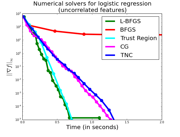
Here, the Trust Region and L-BFGS solver perform almost equally good, with Conjugate Gradient and Truncated Newton falling shortly behind. I was surprised by the difference between BFGS and L-BFGS, I would have thought that when memory was not an issue both algorithms should perform similarly.

To make things more interesting, we now make the design to be slightly more correlated. We do so by adding a constant term of 1 to the matrix $X$ and adding also a column vector of ones this matrix to account for the intercept. These are the results:

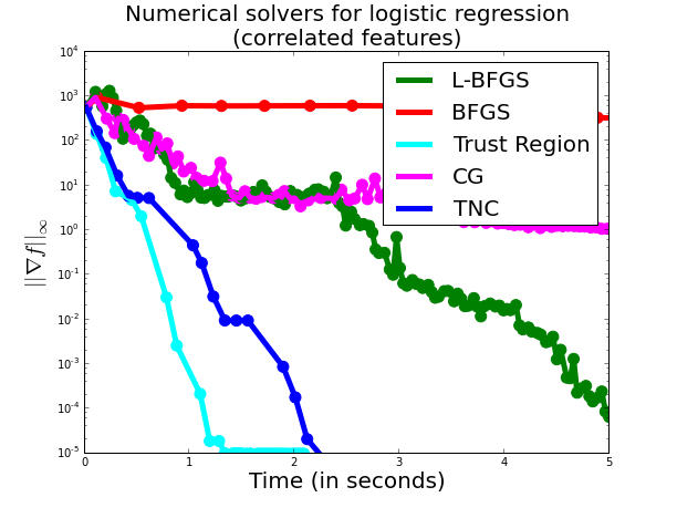
Here, we already see that second-order methods dominate over first-order methods (well, except for BFGS), with Trust Region clearly dominating the picture but with TNC not far behind.

Finally, if we force the matrix to be even more correlated (we add 10. to the design matrix $X$), then we have:

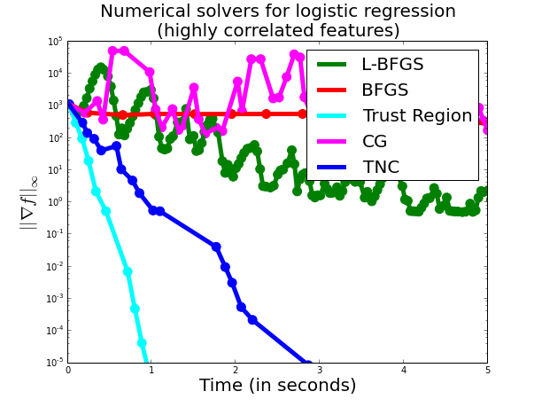
Here, the Trust-Region method has the same timing as before, but all other methods have got substantially worse.The Trust Region method, unlike the other methods is surprisingly robust to correlated designs.

To sum up, the Trust Region method performs extremely well for optimizing the Logistic Regression model under different conditionings of the design matrix. The LIBLINEAR software uses this solver and thus has similar performance, with the sole exception that the evaluation of the logistic function and its derivatives is done in C++ instead of Python. In practice, however, due to the small number of iterations of this solver I haven't seen any significant difference.