TL;DR: I've implemented a logistic ordinal regression or proportional odds model. Here is the Python code

The logistic ordinal regression model, also known as the proportional odds was introduced in the early 80s by McCullagh [¹, ²] and is a generalized linear model specially tailored for the case of predicting ordinal variables, that is, variables that are discrete (as in classification) but which can be ordered (as in regression). It can be seen as an extension of the logistic regression model to the ordinal setting.

Given $X \in \mathbb{R}^{n \times p}$ input data and $y \in \mathbb{N}^n$ target values. For simplicity we assume $y$ is a non-decreasing vector, that is, $y_1 \leq y_2 \leq ...$. Just as the logistic regression models posterior probability $P(y=j|X_i)$ as the logistic function, in the logistic ordinal regression we model the cummulative probability as the logistic function. That is,

$$ P(y \leq j|X_i) = \phi(\theta_j - w^T X_i) = \frac{1}{1 + \exp(w^T X_i - \theta_j)} $$

where $w, \theta$ are vectors to be estimated from the data and $\phi$ is the logistic function defined as $\phi(t) = 1 / (1 + \exp(-t))$.

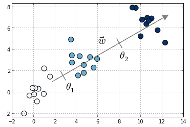
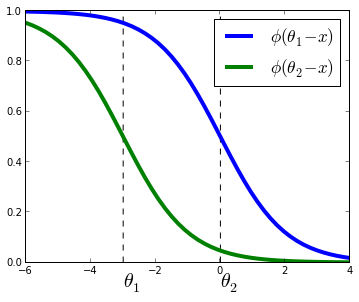
Compared to multiclass logistic regression, we have added the constrain that the hyperplanes that separate the different classes are parallel for all classes, that is, the vector $w$ is common across classes. To decide to which class will $X_i$ be predicted we make use of the vector of thresholds $\theta$. If there are $K$ different classes, $\theta$ is a non-decreasing vector (that is, $\theta_1 \leq \theta_2 \leq ... \leq \theta_{K-1}$) of size $K-1$. We will then assign the class $j$ if the prediction $w^T X$ (recall that it's a linear model) lies in the interval $[\theta_{j-1}, \theta_{j}[$. In order to keep the same definition for extremal classes, we define $\theta_{0} = - \infty$ and $\theta_K = + \infty$.

The intuition is that we are seeking a vector $w$ such that $X w$ produces a set of values that are well separated into the different classes by the different thresholds $\theta$. We choose a logistic function to model the probability $P(y \leq j|X_i)$ but other choices are possible. In the proportional hazards model ¹ the probability is modeled as $-\log(1 - P(y \leq j | X_i)) = \exp(\theta_j - w^T X_i)$. Other link functions are possible, where the link function satisfies $\text{link}(P(y \leq j | X_i)) = \theta_j - w^T X_i$. Under this framework, the logistic ordinal regression model has a logistic link function and the proportional hazards model has a log-log link function.

The logistic ordinal regression model is also known as the proportional odds model, because the ratio of corresponding odds for two different samples $X_1$ and $X_2$ is $\exp(w^T(X_1 - X_2))$ and so does not depend on the class $j$ but only on the difference between the samples $X_1$ and $X_2$.

Optimization

Model estimation can be posed as an optimization problem. Here, we minimize the loss function for the model, defined as minus the log-likelihood:

$$ \mathcal{L}(w, \theta) = - \sum_{i=1}^n \log(\phi(\theta_{y_i} - w^T X_i) - \phi(\theta_{y_i -1} - w^T X_i)) $$

In this sum all terms are convex on $w$, thus the loss function is convex over $w$. It might be also jointly convex over $w$ and $\theta$, although I haven't checked. I use the function fmin_slsqp in scipy.optimize to optimize $\mathcal{L}$ under the constraint that $\theta$ is a non-decreasing vector. There might be better options, I don't know. If you do know, please leave a comment!.

Using the formula $\log(\phi(t))^\prime = (1 - \phi(t))$, we can compute the gradient of the loss function as

$\begin{align} \nabla_w \mathcal{L}(w, \theta) &= \sum_{i=1}^n X_i (1 - \phi(\theta_{y_i} - w^T X_i) - \phi(\theta_{y_i-1} - w^T X_i)) \\ % \nabla_\theta \mathcal{L}(w, \theta) &= \sum_{i=1}^n - \frac{e_{y_i} \exp(\theta_{y_i}) - e_{y_i -1} \exp(\theta_{y_i -1})}{\exp(\theta_{y_i}) - \exp(\theta_{y_i-1})} \\ \nabla_\theta \mathcal{L}(w, \theta) &= \sum_{i=1}^n e_{y_i} \left(1 - \phi(\theta_{y_i} - w^T X_i) - \frac{1}{1 - \exp(\theta_{y_i -1} - \theta_{y_i})}\right) \\ & \qquad + e_{y_i -1}\left(1 - \phi(\theta_{y_i -1} - w^T X_i) - \frac{1}{1 - \exp(- (\theta_{y_i-1} - \theta_{y_i}))}\right) \end{align}$

where $e_i$ is the $i$th canonical vector.

Code

I've implemented a Python version of this algorithm using Scipy's optimize.fmin_slsqp function. This takes as arguments the loss function, the gradient denoted before and a function that is > 0 when the inequalities on $\theta$ are satisfied.

Code can be found here as part of the minirank package, which is my sandbox for code related to ranking and ordinal regression. At some point I would like to submit it to scikit-learn but right now the I don't know how the code will scale to medium-scale problems, but I suspect not great. On top of that I'm not sure if there is a real demand of these models for scikit-learn and I don't want to bloat the package with unused features.

Performance

I compared the prediction accuracy of this model in the sense of mean absolute error (IPython notebook) on the boston house-prices dataset. To have an ordinal variable, I rounded the values to the closest integer, which gave me a problem of size 506 $\times$ 13 with 46 different target values. Although not a huge increase in accuracy, this model did give me better results on this particular dataset:

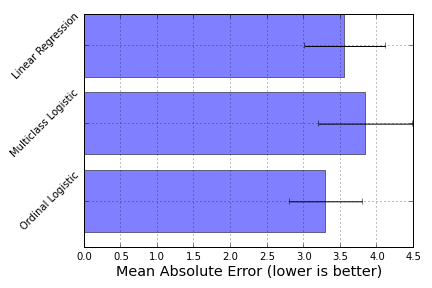
Here, ordinal logistic regression is the best-performing model, followed by a Linear Regression model and a One-versus-All Logistic regression model as implemented in scikit-learn.