SciPy contains two methods to compute the singular value decomposition (SVD) of a matrix: scipy.linalg.svd and scipy.sparse.linalg.svds. In this post I'll compare both methods for the task of computing the full SVD of a large dense matrix.

The first method, scipy.linalg.svd, is perhaps the best known and uses the linear algebra library LAPACK to handle the computations. This implements the Golub-Kahan-Reisch algorithm ¹, which is accurate and highly efficient with a cost of O(n^3) floating-point operations ².

The second method is scipy.sparse.linalg.svds and despite it's name it works fine also for dense arrays. This implementation is based on the ARPACK library and consists of an iterative procedure that finds the SVD decomposition by reducing the problem to an eigendecomposition on the array X -> dot(X.T, X). This method is usually very effective when the input matrix X is sparse or only the largest singular values are required. There are other SVD solvers that I did not consider, such as sparsesvd or pysparse.jdsym, but my points for the sparse solve probably hold for those packages too since they both implement iterative algorithms based on the same principles.

When the input matrix is dense and all the singular values are required, the first method is usually more efficient. To support this statement I've created a little benchmark: timings for both methods as a function of the size of the matrices. Notice that we are in a case that is clearly favorable to the linalg.svd: after all sparse.linalg.svds was not created with this setting in mind, it was created for sparse matrices or dense matrices with some special structure. We will see however that even in this setting it has interesting advantages.

I'll create random square matrices with different sizes and plot the timings for both methods. For the benchmarks I used SciPy v0.12 linked against Intel Math Kernel Library v11. Both methods are single-threaded (I had to set OMP_NUM_THREADS=1 so that MKL does not try to parallelize the computations). [code]

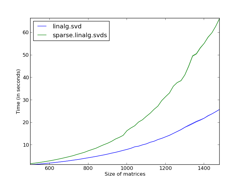
Lower timings are better, so this gives scipy.linalg.svd as clear winner. However, this is just part of the story. What this graph doesn't show is that this method is winning at the price of allocating a huge amount of memory for temporary computations. If we now plot the memory consumption for both methods under the same settings, the story is completely different. [code]

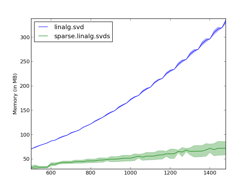
The memory requirements of scipy.linalg.svd scale with the number of dimensions, while for the sparse version the amount of allocated memory is constant. Notice that we are measuring the amount of total memory used, it is thus natural to see a slight increase in memory consumption since the input matrix is bigger on each iteration.

For example, in my applications, I need to compute the SVD of a matrix for whom the needed workspace does not fit in memory. In cases like this, the sparse algorithm (sparse.linalg.svds) can come in handy: the timing is just a factor worse (but I can easily parallelize jobs) and the memory requirements for this method is peanuts compared to the dense version.