A naive implementation of the logistic regression loss can results in numerical indeterminacy even for moderate values. This post takes a closer look into the source of these instabilities and discusses more robust Python implementations.

Logistic regression

Consider the logistic regression loss, defined as \begin{equation}\label{eq:logloss} f(\xx) \defas \frac{1}{n}\sum_{i=1}^n - b_i \log(s(\aa_i^\intercal \xx)) - (1 - b_i) \log(1 - s(\aa_i^\intercal \xx))~, \end{equation} where each $\aa_i$ is a $d$-dimensional vector, $b_i$ is a scalar between 0 and 1, and $s(t) \defas 1 / (1 + \exp(-t))$ is the sigmoid function. My goal in this post will be to derive Python code that can evaluate this function as precisely as possible without sacrificing speed.Some references use the following slightly different formulation \begin{equation} \label{eq:logloss2} \frac{1}{n}\sum_{i=1}^n \log(c_i s(\aa_i^\intercal \xx))~, \end{equation} where $c_i$ is a scalar that takes the value -1 when $b_i = 0$ or and 1 when $b_i = 1$. That both formulations are equivalent is not obvious but can be proven by a distinction of cases on $b_i$. This is the formulation that appears for example in the scikit-learn documentation. This function has many interpretations that we will not go into here, as my main focus will be the numerical issues that arise when evaluating this expression.

Below is a straightforward implementation of the previous equation, where $A$ is the row-wise stacking of $\aa_i$:

import numpy as np


def f_naive(x, A, b):
    """Logistic loss, naive implementation."""
    z = np.dot(A, x)
    tmp = 1. / (1 + np.exp(-z))
    return np.mean(- b * np.log(tmp) - (1 - b) * np.log(1 - tmp))

It turns out that this simple and innocent-looking implementation will overflow for moderately large values of the input. This can be a real problem for example when training a machine learning model that uses this loss function.Luckily, most machine learning libraries provide more sophisticated implementations that can safeguard against this indeterminacy. I (Fabian) first saw this tricks in the liblinear package around 2010, although the trick was likely known and used even before. In this library, the implementation of the logistic loss contains a distinction of cases to safeguard from the indeterminacy. For example, if we try the above code with inputs (say) $A = [[1, 1]], b=[1]$ and $x=[20, 20]$ we get the dreadful Not-A-Number (NaN):

>>> A = [[1, 1]]
>>> b = [1]
>>> f_naive([20, 20], A, b)
RuntimeWarning: divide by zero encountered in log
RuntimeWarning: invalid value encountered in multiply
nan

This happens because the two terms in 1 + np.exp(-z) are on very different scales. exp(-40) is of the order of $10^{-18}$. Since double precision can hold up to 17 significant decimal digits, the expression 1 + np.exp(-40) gets truncated to 1, a phenomenon known as round-off error in numerical analysis.

Second, the exponential function will overflow for large values of the input. For double precision types (float64 in NumPy jargon), $e^t$ overflows for values $t \geq 710$, while for single precision types (float32) this happens for $t \geq 89$.

A closer look at the log-sigmoid

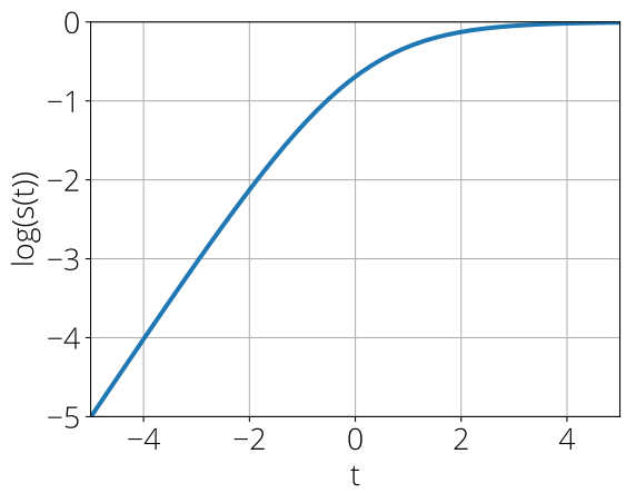Log-sigmoid function in the interval [-5, 5]. The issues encountered before happen during the evaluation of the log-sigmoid function $\log(s(\cdot))$. Therefore we take a closer look into this function and examine its accuracy. We will compare the following 3 different implementations:

1. naive. Directly evaluating $\log(s(t))$ as in the previous implementation. In code, this corresponds to

import numpy as np

def logsig_naive(t):
    return np.log(1 / (1 + np.exp(-t)))

2. logsumexp. Scipy's logsumexp computes the expression \begin{equation} \varphi(\bb) = \log\left(\sum^{d}_{i=1} \exp(b_i)\right)~. \end{equation} We can reuse this function to compute the log-sigmoid through the identity \begin{align} \log(s(t)) &= \log(1/(1 + \exp(-t)))\\ &= -\log(1 + \exp(-t))\\ &= - \varphi([0, -t])~. \end{align} This suggests the following implementation:

import numpy as np
from scipy import special

def logsig_logsumexp(t):
    return - special.logsumexp([0, -t])

3. log1pexp. Martin Mächler wrote a note in 2012 on how to compute accurately the log-sigmoid function in the R language. His technique is based on using different approximations for different values of the input and uses the np.log1p function, which computes $\log(1 + x)$ for small values of $x$. This implementation of the log-sigmoid function is \begin{equation} \log(s(t)) = \begin{cases} t & t < -33.3\\ t - \exp(t) & -33.3 \leq t \leq -18 \\ -\text{log1p}(\exp(-t)) & -18 \leq t \leq 37 \\ -\exp(-t) & 37 \leq t\\ \end{cases}~. \end{equation} A Python implementation of this could be

import numpy as np

def logsig_log1pexp(t):
    if t < -33.3:
        return t
    elif t <= -18:
        return t - np.exp(t)
    elif t <= 37:
        return -np.log1p(np.exp(-t))
    else:
        return -np.exp(-t)

We now would like to compare the different methods. For this, we look at the relative error \begin{equation} \frac{y - \widehat{y}}{y}~, \end{equation} where $\hat{y}$ is the value computed by the method we want to evaluate and $y$ is the true value, computed in this case using mpmath, a library for arbitrary precision arithmetic. The plot below shows this relative accuracy (lower is better) for the previous methods and over a wide range of inputs:

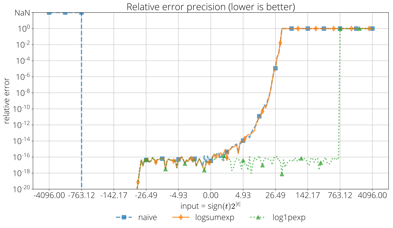
Relative precision for the logistic loss computation (lower is better). While most methods do reasonably well for negative values, the precision quickly deteriorates in the positive regime. Values above 1 indicate that the routine gave NaN.

This plot shows that the log1pexp indeed has a much greater accuracy than the alternative implementations. It also shows the poor accuracy of logsumexp in the positive domain. We found this surprising since we were expecting scipy's logsumexp to provide a more accurate evaluation of the log-sum-exp expression. While its true that it does not suffer from overflow, other than that it doesn't provide a more accurate implementation than the naive implementation.

TL;DR: Use log1pexp. The naive implementation will overflow and give poor accuracy, logsumexp will yield a poor accuracy. log1pexp suffers from these issues the least.

A more stable implementation of the logistic loss

With the results from the previous section we can now write a more stable version of the logistic loss.

One last trick that we will use is to use the formula $\log(1 - s(z)) = -z + \log(s(z))$ to simplify \eqref{eq:logloss} slightly so that it becomes \begin{equation}\label{eq:logistic2} f(\xx) = \frac{1}{n}\sum_{i=1}^n (1 - b_i) \aa_i^\intercal \xx - \log(s(\aa_i^\intercal \xx))~. \end{equation}

And finally, here is the full Python implementation. The routine logsig is slightly more convoluted that the ones presented before because it performs the previous routine component-wise without for loops for efficiency on large arrays:

import numpy as np
from scipy import special


def logsig(x):
    """Compute the log-sigmoid function component-wise."""
    out = np.zeros_like(x)
    idx0 = x < -33
    out[idx0] = x[idx0]
    idx1 = (x >= -33) & (x < -18)
    out[idx1] = x[idx1] - np.exp(x[idx1])
    idx2 = (x >= -18) & (x < 37)
    out[idx2] = -np.log1p(np.exp(-x[idx2]))
    idx3 = x >= 37
    out[idx3] = -np.exp(-x[idx3])
    return out


def f(x, A, b):
    """Logistic loss, numerically stable implementation.
    
    Parameters
    ----------
    x: array-like, shape (n_features,)
        Coefficients

    A: array-like, shape (n_samples, n_features)
        Data matrix

    b: array-like, shape (n_samples,)
        Labels

    Returns
    -------
    loss: float
    """
    z = np.dot(A, x)
    b = np.asarray(b)
    return np.mean((1 - b) * z - logsig(z))

In the same example as before, this implementation does not overflow anymore:

>>> A = [[1, 1]]
>>> b = [1]
>>> f([20, 20], A, b)
0.0

Gradient

For optimization, having an accurate evaluation the gradient is crucial to achieve a solution with high accuracy. In this section I'll compare different approaches to compute this gradient.

Computation of the gradient of the logistic loss simplifies considerably thanks to the following identity verified by the sigmoid function: \begin{equation}\label{eq:diffeq_sigma} \frac{d}{dt}s(t) = s(t)(1 - s(t))~. \end{equation} In particular, this implies that \begin{equation} \label{eq:dif_log} \frac{d}{dt}\log(s(t)) = \frac{\frac{d}{dt}s(t)}{s(t)} = 1 - s(t) \end{equation}

Using these identities and \eqref{eq:logistic2}, we can write the gradient of the logistic loss as \begin{equation} \label{eq:gradient} \nabla f(\xx) =~ \frac{1}{n}\sum_{i=1}^n\aa_i (s(\aa_i^\intercal \xx) - b_i) \end{equation}

As we will see, there are also some numerical issues with the computation of $b_i - s(\cdot)$ that can be problematic when computing this expression. We will now compare three different implementations of $g(t) \defas s(t) - b$:

1. naive. The previous equation is easy to implement using SciPy's sigmoid function (special.expit):

from scipy import special

def g_naive(t, b):
    return special.expit(t) - b
  

Unfortunately, the subtraction of $b_i$ can cause a problematic loss of precision when this is close to 1:

>>> g_naive(40, 1)
0.0
  

while the correct answer is $\approx -4.24 \times 10^{-18}$.

2. g_v2. We can avoid precision loss of the previous example by reformulating the problematic expression into a single fraction as \begin{equation} s(t) - b = \frac{1}{1 + e^{-t}} - b = \frac{(1 - b) - b e^{-t}}{1 + e^{-t}}\label{eq:expit_b} \end{equation} In this case, when $b=1$ the expression becomes $1 / (e^t + 1)$, which doesn't suffer from the same issue.

import numpy as np

def g_v2(t, b):
    exp_nt = np.exp(-t)
    return ((1 - b) - b * exp_nt) / (1 + exp_nt)

Which as advertised gives a more accurate answer in the previous case:

>>> g_v2(40, 1)
-4.248354255291589e-18

While better than the naive approach, this routine suffers from some issues. For example, the exponential will overflow for large values of $t$ (starting around 800), with this routine returning NaN:

>>> g_v2(800, 1)
RuntimeWarning: overflow encountered in exp
RuntimeWarning: invalid value encountered in double_scalars
nan
    

3. g_sign. We can fix this last problem by avoiding to evaluate the exponential function with a large input. For this, we multiply both sides of \eqref{eq:expit_b} by $e^{-t}$ to arrive at the equivalent expression $((1 - b) - b e^{-t}) / (1 + e^{-t})$, which does not have any terms on $e^t$. Finally, we choose this formula whenever $t> 0$ and the previous one otherwise. This gives the following code:

import numpy as np

def g_sign(t, b):
    if t < 0:
        exp_t = np.exp(t)
        return ((1 - b) * exp_t - b) / (1 + exp_t)
    else:
        # same approach as g_v2
        exp_nt = np.exp(-t)
        return ((1 - b) - b * exp_nt) / (1 + exp_nt)

And we can check that this no longer overflows:

>>> g_sign(800, 1)
0.0
  

Comparison

We now compare relative accuracy of these approaches. In the plot below, we show the relative accuracy (lower is better) a function of the input.

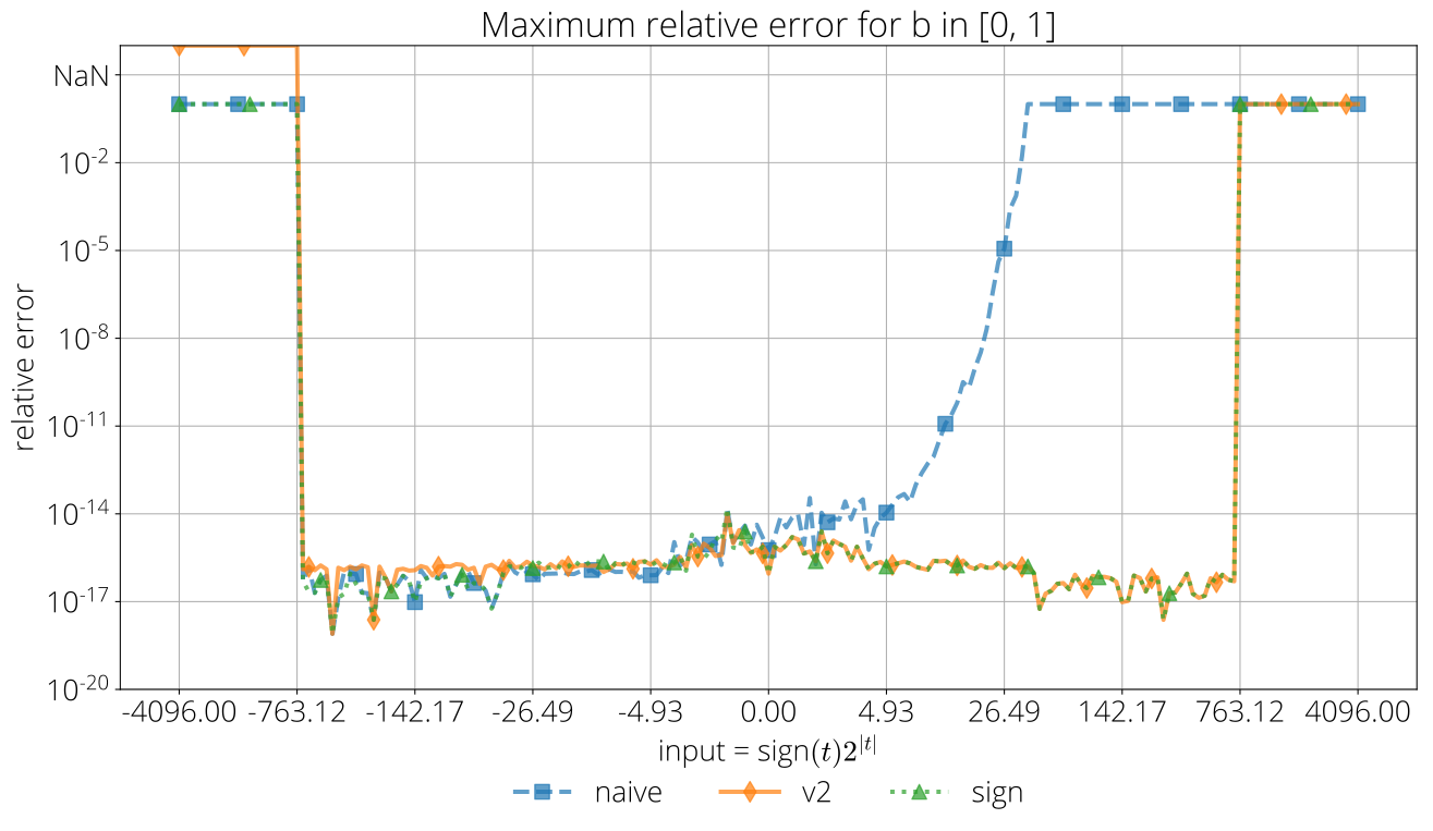
Relative precision for different implementations of the logistic loss's gradient (lower is better).The naive method quickly suffers from relative of precision in the positive segment. expit_b exhibits a better accuracy but outputs NaN for large values of the input (values above 1 indicate NaN). expit_sign has none of these issues and has the best overall accuracy.

This plot shows that the sign version has an accuracy at least as good as the v2 function, minus the indeterminacy for large values of the input.

TL;DR: use g_sign.

A more stable gradient.

We can now use the more stable routines developed in the last section to compute the full gradient. As before, the auxiliary routine (expit_b in this case) is slightly more convoluted that the ones presented before because it performs the previous routine component-wise without for loops for efficiency on large arrays:A full implementation of the logistic loss and its gradients with some bells and whistles like support for sparse matrices (and incidentally, the main motivation for writing this post) can be found in the optimization package copt.

import numpy as np


def expit_b(x, b):
    """Compute sigmoid(x) - b component-wise."""
    idx = x < 0
    out = np.zeros_like(x)
    exp_x = np.exp(x[idx])
    b_idx = b[idx]
    out[idx] = ((1 - b_idx) * exp_x - b_idx) / (1 + exp_x)
    exp_nx = np.exp(-x[~idx])
    b_nidx = b[~idx]
    out[~idx] = ((1 - b_nidx) - b_nidx * exp_nx) / (1 + exp_nx)
    return out


def f_grad(x, A, b):
    """Computes the gradient of the logistic loss.
    
    Parameters
    ----------
    x: array-like, shape (n_features,)
        Coefficients

    A: array-like, shape (n_samples, n_features)
        Data matrix

    b: array-like, shape (n_samples,)
        Labels

    Returns
    -------
    grad: array-like, shape (n_features,)    
    """
    z = A.dot(x)
    s = expit_b(z, b)
    return A.T.dot(s) / A.shape[0] 

Conclusion

A naive coding of the logistic loss and its gradient suffers numerical issues that go from indeterminacy to loss of precision. In this post I compared different approaches that can be used to mitigate this problem. Machine learning software typically implements some of these approaches, as obtaining a single NaN value during training can be fatal. For example, both scikit-learn and tensorflow make a distinction of cases on the sign for the gradient, as the g_sign method above.

A word about speed. The speed difference between the different approaches is almost none for high-dimensional problems since the cost of evaluating the logistic function or its gradient is negligible compared that of the dot vector product $\aa_i^\intercal \xx$. For example, on a 20.000-dimensional square problem, the timing of f and f_naive is almost the same, with a slight difference for the latter since it avoids some evaluations of the log and exp:

>>> A = np.random.randn(2000, 2000)
>>> b = (np.sign(np.random.randn(2000)) + 1) // 2
>>> x = np.random.randn(2000)
>>> %timeit f(x, A, b) 
1.74 ms ± 158 µs per loop (mean ± std. dev. of 7 runs, 1000 loops each)
>>> %timeit f_naive(x, A, b)
1.97 ms ± 338 µs per loop (mean ± std. dev. of 7 runs, 1000 loops each)