





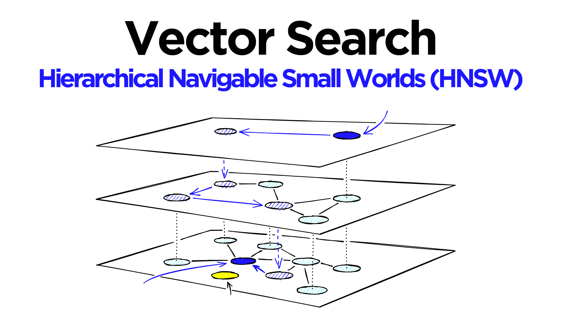
Hierarchical Navigable Small World (HNSW) graphs are among the top-performing indexes for vector similarity search[1]. HNSW is a hugely popular technology that time and time again produces state-of-the-art performance with super fast search speeds and fantastic recall.
Yet despite being a popular and robust algorithm for approximate nearest neighbors (ANN) searches, understanding how it works is far from easy.
Note: Pinecone lets you build scalable, performant vector search into applications without knowing anything about HNSW or vector indexing libraries. But we know you like seeing how things work, so enjoy the guide!
This article helps demystify HNSW and explains this intelligent algorithm in an easy-to-understand way. Towards the end of the article, we’ll look at how to implement HNSW using Faiss and which parameter settings give us the performance we need.
Foundations of HNSW
We can split ANN algorithms into three distinct categories; trees, hashes, and graphs. HNSW slots into the graph category. More specifically, it is a proximity graph, in which two vertices are linked based on their proximity (closer vertices are linked) — often defined in Euclidean distance.
There is a significant leap in complexity from a ‘proximity’ graph to ‘hierarchical navigable small world’ graph. We will describe two fundamental techniques that contributed most heavily to HNSW: the probability skip list, and navigable small world graphs.
Probability Skip List
The probability skip list was introduced way back in 1990 by William Pugh [2]. It allows fast search like a sorted array, while using a linked list structure for easy (and fast) insertion of new elements (something that is not possible with sorted arrays).
Skip lists work by building several layers of linked lists. On the first layer, we find links that skip many intermediate nodes/vertices. As we move down the layers, the number of ‘skips’ by each link is decreased.
To search a skip list, we start at the highest layer with the longest ‘skips’ and move along the edges towards the right (below). If we find that the current node ‘key’ is greater than the key we are searching for — we know we have overshot our target, so we move down to previous node in the next level.
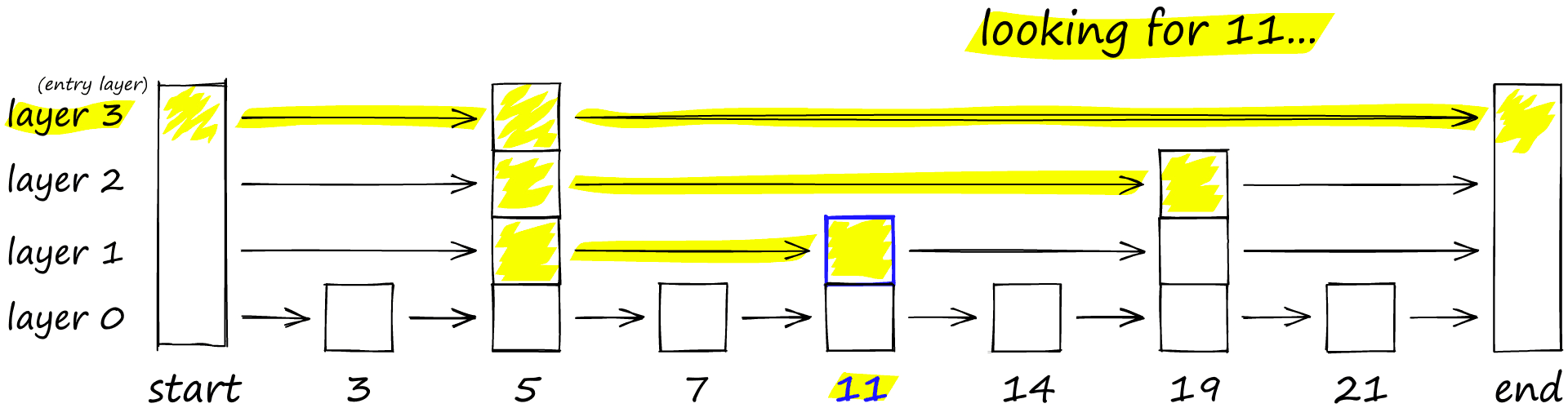
A probability skip list structure, we start on the top layer. If our current key is greater than the key we are searching for (or we reach end), we drop to the next layer.
HNSW inherits the same layered format with longer edges in the highest layers (for fast search) and shorter edges in the lower layers (for accurate search).
Navigable Small World Graphs
Vector search using Navigable Small World (NSW) graphs was introduced over the course of several papers from 2011-14 [4, 5, 6]. The idea is that if we take a proximity graph but build it so that we have both long-range and short-range links, then search times are reduced to (poly/)logarithmic complexity.
Each vertex in the graph connects to several other vertices. We call these connected vertices friends, and each vertex keeps a friend list, creating our graph.
When searching an NSW graph, we begin at a pre-defined entry-point. This entry point connects to several nearby vertices. We identify which of these vertices is the closest to our query vector and move there.
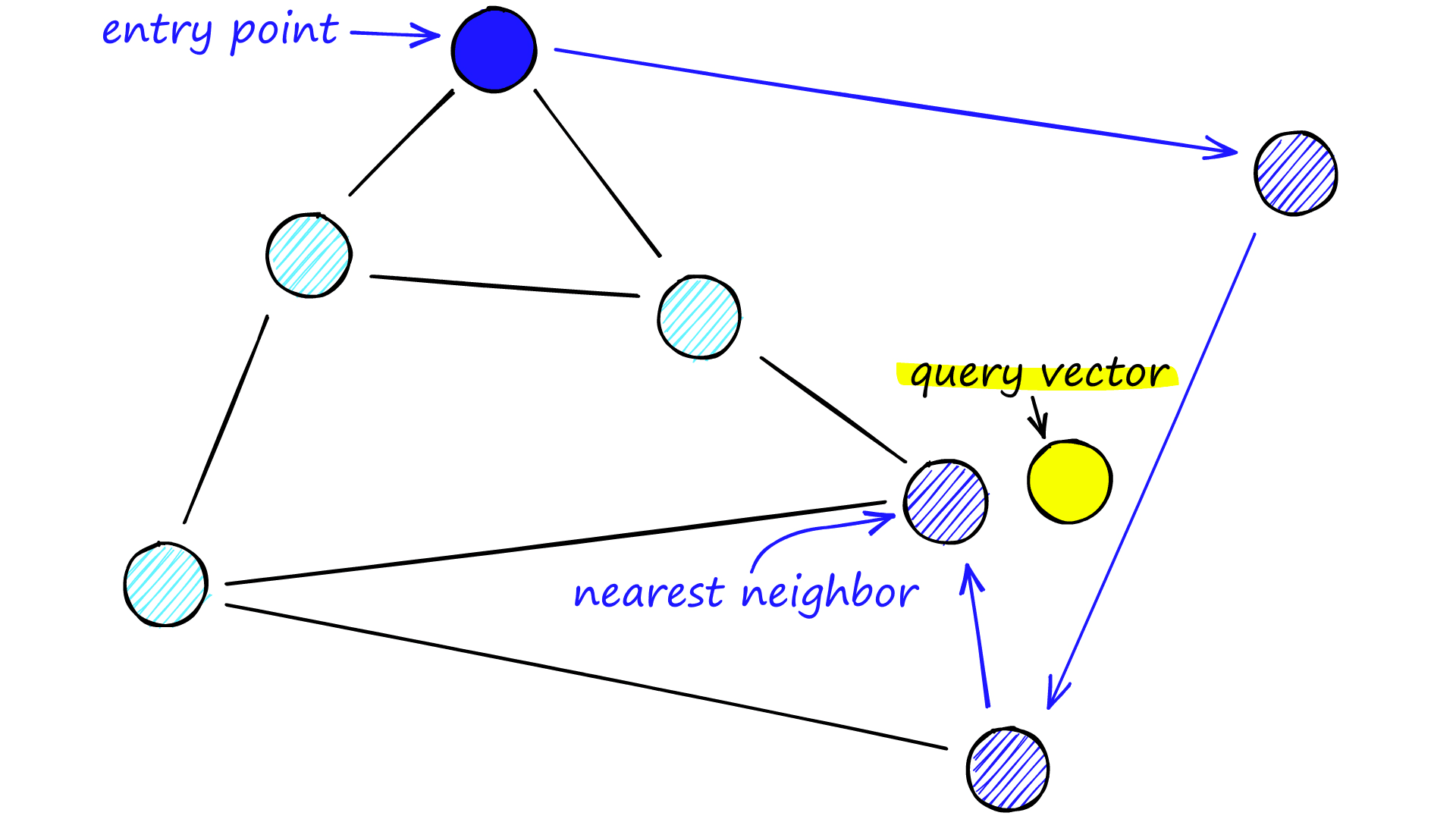
The search process through a NSW graph. Starting at a pre-defined entry point, the algorithm greedily traverses to connected vertices that are nearer to the query vector.
We repeat the greedy-routing search process of moving from vertex to vertex by identifying the nearest neighboring vertices in each friend list. Eventually, we will find no nearer vertices than our current vertex — this is a local minimum and acts as our stopping condition.
Navigable small world models are defined as any network with (poly/)logarithmic complexity using greedy routing. The efficiency of greedy routing breaks down for larger networks (1-10K+ vertices) when a graph is not navigable [7].
The routing (literally the route we take through the graph) consists of two phases. We start with the “zoom-out” phase where we pass through low-degree vertices (degree is the number of links a vertex has) — and the later “zoom-in” phase where we pass through higher-degree vertices [8].
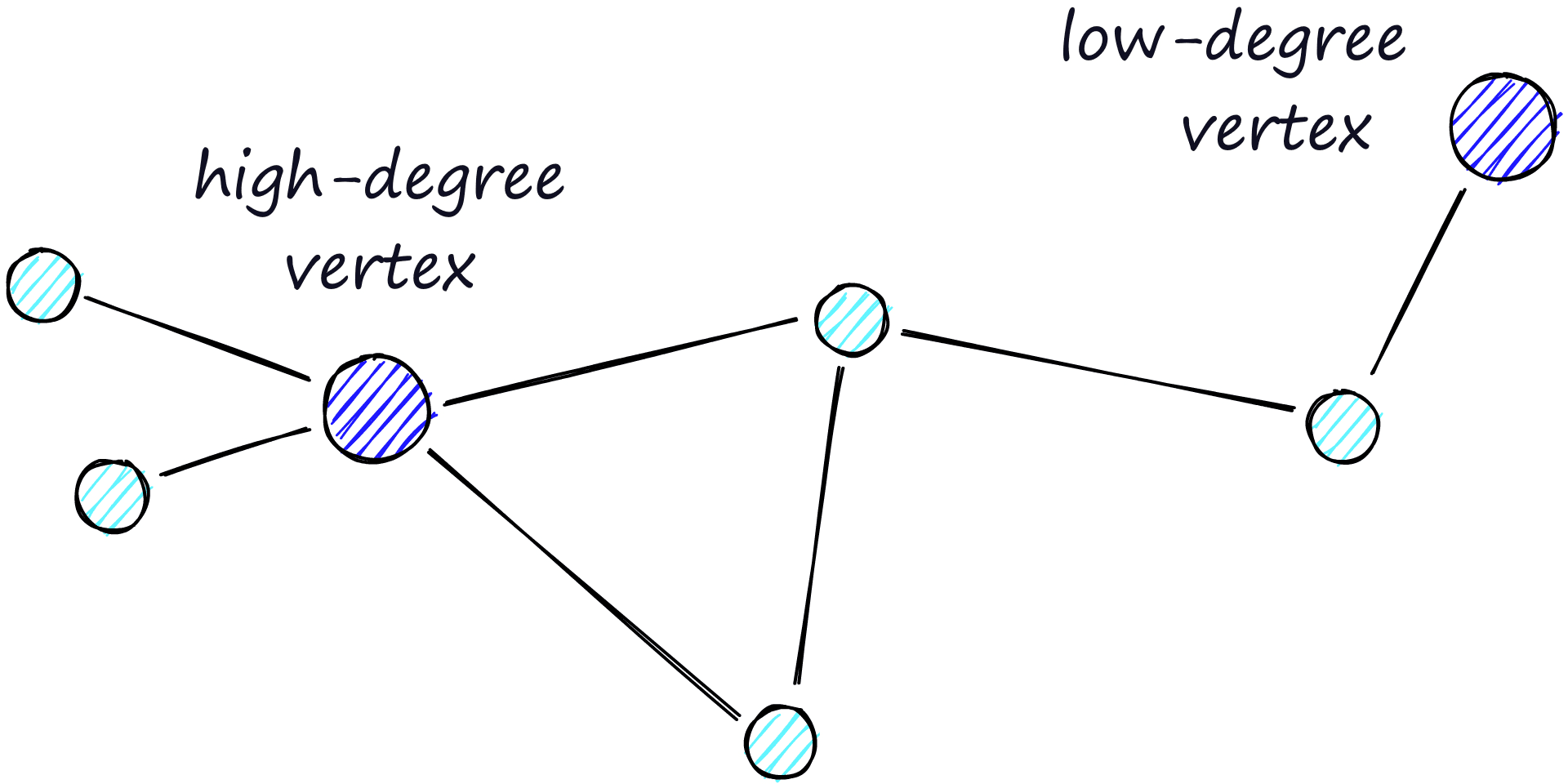
High-degree vertices have many links, whereas low-degree vertices have very few links.
Our stopping condition is finding no nearer vertices in our current vertex’s friend list. Because of this, we are more likely to hit a local minimum and stop too early when in the zoom-out phase (fewer links, less likely to find a nearer vertex).
To minimize the probability of stopping early (and increase recall), we can increase the average degree of vertices, but this increases network complexity (and search time). So we need to balance the average degree of vertices between recall and search speed.
Another approach is to start the search on high-degree vertices (zoom-in first). For NSW, this does improve performance on low-dimensional data. We will see that this is also a significant factor in the structure of HNSW.
Creating HNSW
HNSW is a natural evolution of NSW, which borrows inspiration from hierarchical multi-layers from Pugh’s probability skip list structure.
Adding hierarchy to NSW produces a graph where links are separated across different layers. At the top layer, we have the longest links, and at the bottom layer, we have the shortest.
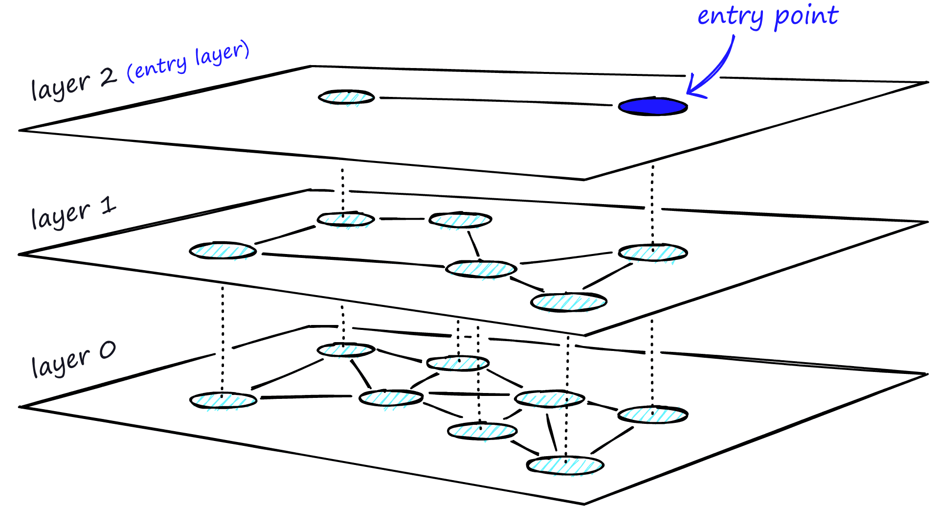
Layered graph of HNSW, the top layer is our entry point and contains only the longest links, as we move down the layers, the link lengths become shorter and more numerous.
During the search, we enter the top layer, where we find the longest links. These vertices will tend to be higher-degree vertices (with links separated across multiple layers), meaning that we, by default, start in the zoom-in phase described for NSW.
We traverse edges in each layer just as we did for NSW, greedily moving to the nearest vertex until we find a local minimum. Unlike NSW, at this point, we shift to the current vertex in a lower layer and begin searching again. We repeat this process until finding the local minimum of our bottom layer — layer 0.
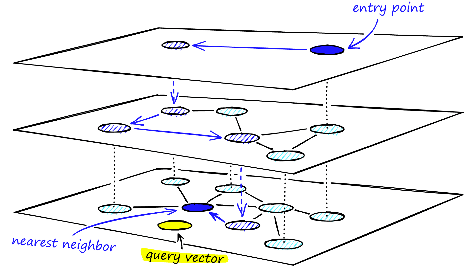
The search process through the multi-layer structure of an HNSW graph.
Graph Construction
During graph construction, vectors are iteratively inserted one-by-one. The number of layers is represented by parameter L. The probability of a vector insertion at a given layer is given by a probability function normalized by the ‘level multiplier’ m_L, where m_L = ~0 means vectors are inserted at layer 0 only.
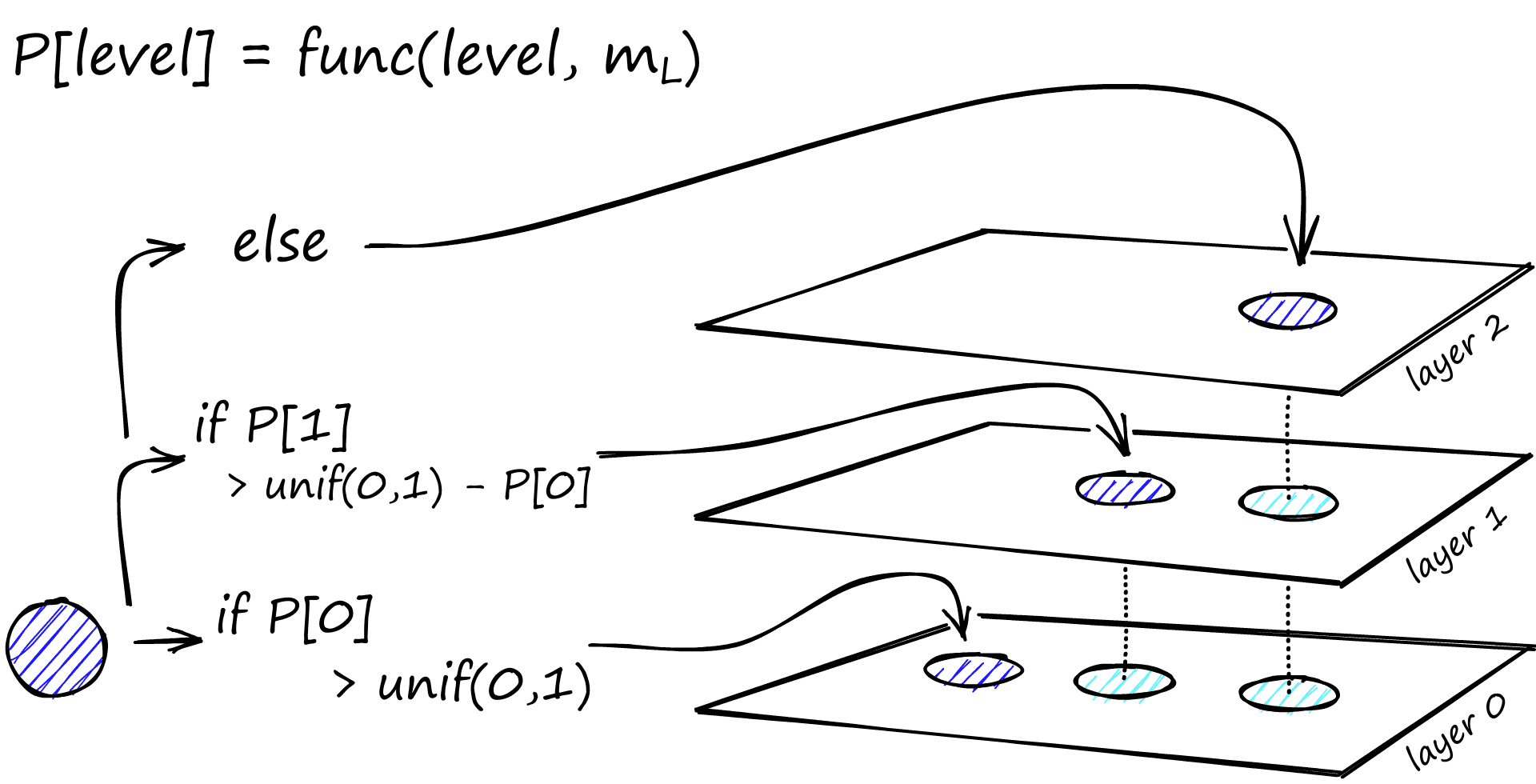
The probability function is repeated for each layer (other than layer 0). The vector is added to its insertion layer and every layer below it.
The creators of HNSW found that the best performance is achieved when we minimize the overlap of shared neighbors across layers. Decreasing m_L can help minimize overlap (pushing more vectors to layer 0), but this increases the average number of traversals during search. So, we use an m_L value which balances both. A rule of thumb for this optimal value is 1/ln(M) [1].
Graph construction starts at the top layer. After entering the graph the algorithm greedily traverse across edges, finding the ef nearest neighbors to our inserted vector q — at this point ef = 1.
After finding the local minimum, it moves down to the next layer (just as is done during search). This process is repeated until reaching our chosen insertion layer. Here begins phase two of construction.
The ef value is increased to efConstruction (a parameter we set), meaning more nearest neighbors will be returned. In phase two, these nearest neighbors are candidates for the links to the new inserted element q and as entry points to the next layer.
M neighbors are added as links from these candidates — the most straightforward selection criteria are to choose the closest vectors.
After working through multiple iterations, there are two more parameters that are considered when adding links. M_max, which defines the maximum number of links a vertex can have, and M_max0, which defines the same but for vertices in layer 0.
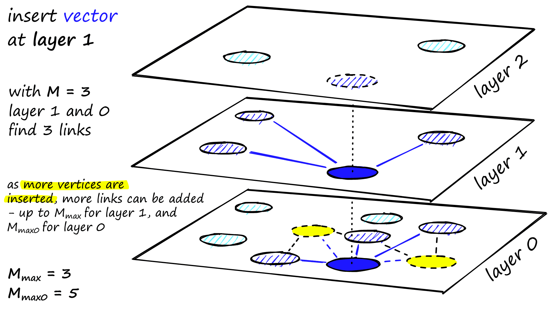
Explanation of the number of links assigned to each vertex and the effect of M, M_max, and M_max0.
The stopping condition for insertion is reaching the local minimum in layer 0.
Implementation of HNSW
We will implement HNSW using the Facebook AI Similarity Search (Faiss) library, and test different construction and search parameters and see how these affect index performance.
To initialize the HNSW index we write:
In[2]:
# setup our HNSW parameters
d = 128  # vector size
M = 32

index = faiss.IndexHNSWFlat(d, M)
print(index.hnsw)
Out[2]:
<faiss.swigfaiss.HNSW; proxy of <Swig Object of type 'faiss::HNSW *' at 0x7f91183ef120> >
With this, we have set our M parameter — the number of neighbors we add to each vertex on insertion, but we’re missing M_max and M_max0.
In Faiss, these two parameters are set automatically in the set_default_probas method, called at index initialization. The M_max value is set to M, and M_max0 set to M*2 (find further detail in the notebook).
Before building our index with index.add(xb), we will find that the number of layers (or levels in Faiss) are not set:
In[3]:
# the HNSW index starts with no levels
index.hnsw.max_level
In[4]:
# and levels (or layers) are empty too
levels = faiss.vector_to_array(index.hnsw.levels)
np.bincount(levels)
If we go ahead and build the index, we’ll find that both of these parameters are now set.
In[6]:
# after adding our data we will find that the level
# has been set automatically
index.hnsw.max_level
In[7]:
# and levels (or layers) are now populated
levels = faiss.vector_to_array(index.hnsw.levels)
np.bincount(levels)
Out[7]:
array([ 0, 968746, 30276, 951, 26, 1], dtype=int64)Here we have the number of levels in our graph, 0 -> 4 as described by max_level. And we have levels, which shows the distribution of vertices on each level from 0 to 4 (ignoring the first 0 value). We can even find which vector is our entry point:
That’s a high-level view of our Faiss-flavored HNSW graph, but before we test the index, let’s dive a little deeper into how Faiss is building this structure.
Graph Structure
When we initialize our index we pass our vector dimensionality d and number of neighbors for each vertex M. This calls the method ‘set_default_probas’, passing M and 1 / log(M) in the place of levelMult (equivalent to m_L above). A Python equivalent of this method looks like:
def set_default_probas(M: int, m_L: float):
    nn = 0  # set nearest neighbors count = 0
    cum_nneighbor_per_level = []
    level = 0  # we start at level 0
    assign_probas = []
    while True:
        # calculate probability for current level
        proba = np.exp(-level / m_L) * (1 - np.exp(-1 / m_L))
        # once we reach low prob threshold, we've created enough levels
        if proba < 1e-9: break
        assign_probas.append(proba)
        # neighbors is == M on every level except level 0 where == M*2
        nn += M*2 if level == 0 else M
        cum_nneighbor_per_level.append(nn)
        level += 1
    return assign_probas, cum_nneighbor_per_level
Here we are building two vectors — assign_probas, the probability of insertion at a given layer, and cum_nneighbor_per_level, the cumulative total of nearest neighbors assigned to a vertex at different insertion levels.
In[10]:
assign_probas, cum_nneighbor_per_level = set_default_probas(
    32, 1/np.log(32)
)
assign_probas, cum_nneighbor_per_level
Out[10]:
([0.96875,
  0.030273437499999986,
  0.0009460449218749991,
  2.956390380859371e-05,
  9.23871994018553e-07,
  2.887099981307982e-08],
 [64, 96, 128, 160, 192, 224])
From this, we can see the significantly higher probability of inserting a vector at level 0 than higher levels (although, as we will explain below, the probability is not exactly as defined here). This function means higher levels are more sparse, reducing the likelihood of ‘getting stuck’, and ensuring we start with longer range traversals.
Our assign_probas vector is used by another method called random_level — it is in this function that each vertex is assigned an insertion level.
def random_level(assign_probas: list, rng):
    # get random float from 'r'andom 'n'umber 'g'enerator
    f = rng.uniform()
    for level in range(len(assign_probas)):
        # if the random float is less than level probability...
        if f < assign_probas[level]:
            # ... we assert at this level
            return level
        # otherwise subtract level probability and try again
        f -= assign_probas[level]
    # below happens with very low probability
    return len(assign_probas) - 1
We generate a random float using Numpy’s random number generator rng (initialized below) in f. For each level, we check if f is less than the assigned probability for that level in assign_probas — if so, that is our insertion layer.
If f is too high, we subtract the assign_probas value from f and try again for the next level. The result of this logic is that vectors are most likely going to be inserted at level 0. Still, if not, there is a decreasing probability of insertion at ease increment level.
Finally, if no levels satisfy the probability condition, we insert the vector at the highest level with return len(assign_probas) - 1. If we compare the distribution between our Python implementation and that of Faiss, we see very similar results:
In[12]:
chosen_levels = []
rng = np.random.default_rng(12345)
for _ in range(1_000_000):
    chosen_levels.append(random_level(assign_probas, rng))
In[13]:
np.bincount(chosen_levels)Out[13]:
array([968821,  30170,    985,     23,       1],
      dtype=int64)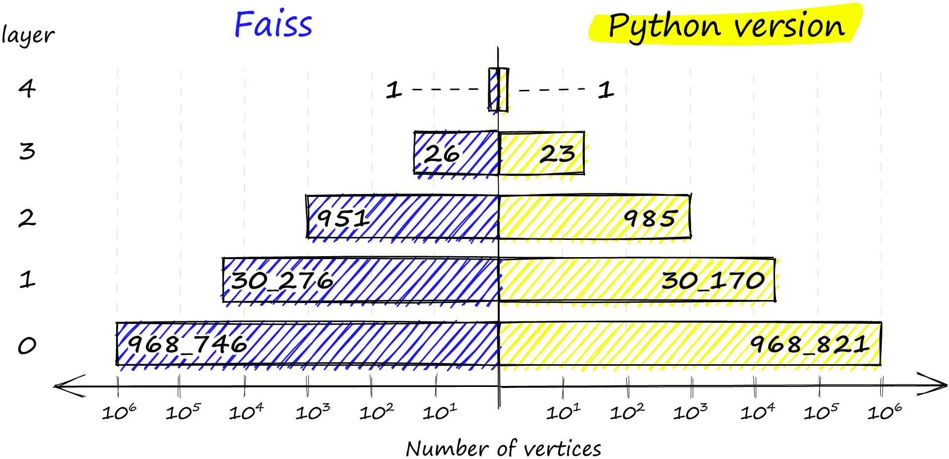
Distribution of vertices across layers in both the Faiss implementation (left) and the Python implementation (right).
The Faiss implementation also ensures that we always have at least one vertex in the highest layer to act as the entry point to our graph.
HNSW Performance
Now that we’ve explored all there is to explore on the theory behind HNSW and how this is implemented in Faiss — let’s look at the effect of different parameters on our recall, search and build times, and the memory usage of each.
We will be modifying three parameters: M, efSearch, and efConstruction. And we will be indexing the Sift1M dataset, which you can download and prepare using this script.
As we did before, we initialize our index like so:
index = faiss.IndexHNSWFlat(d, M)The two other parameters, efConstruction and efSearch can be modified after we have initialized our index.
index.hnsw.efConstruction = efConstruction
index.add(xb)  # build the index
index.hnsw.efSearch = efSearch
# and now we can search
index.search(xq[:1000], k=1)
Our efConstruction value must be set before we construct the index via index.add(xb), but efSearch can be set anytime before searching.
Let’s take a look at the recall performance first.
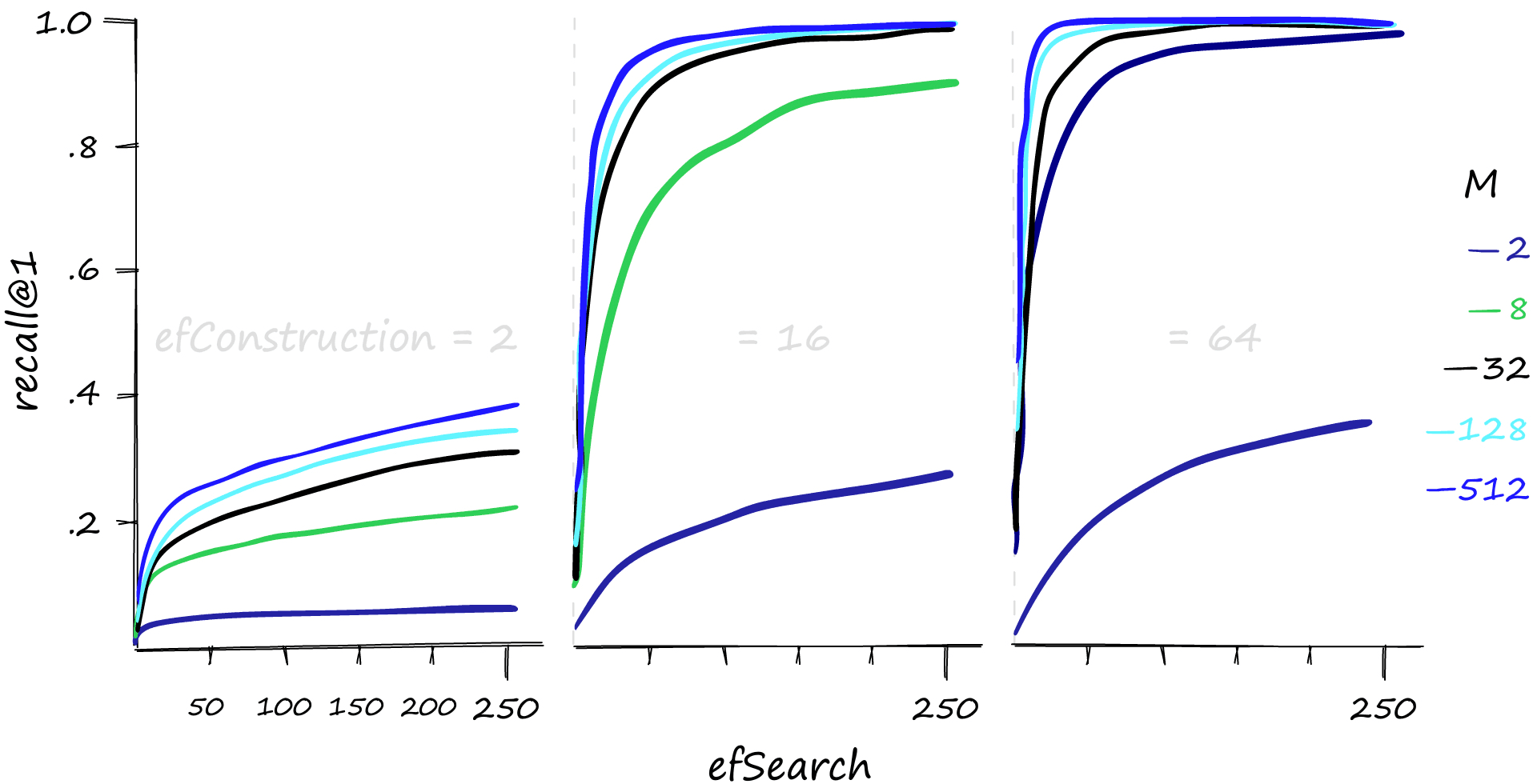
Recall@1 performance for various M, efConstruction, and efSearch parameters.
High M and efSearch values can make a big difference in recall performance — and it’s also evident that a reasonable efConstruction value is needed. We can also increase efConstruction to achieve higher recall at lower M and efSearch values.
However, this performance does not come for free. As always, we have a balancing act between recall and search time — let’s take a look.
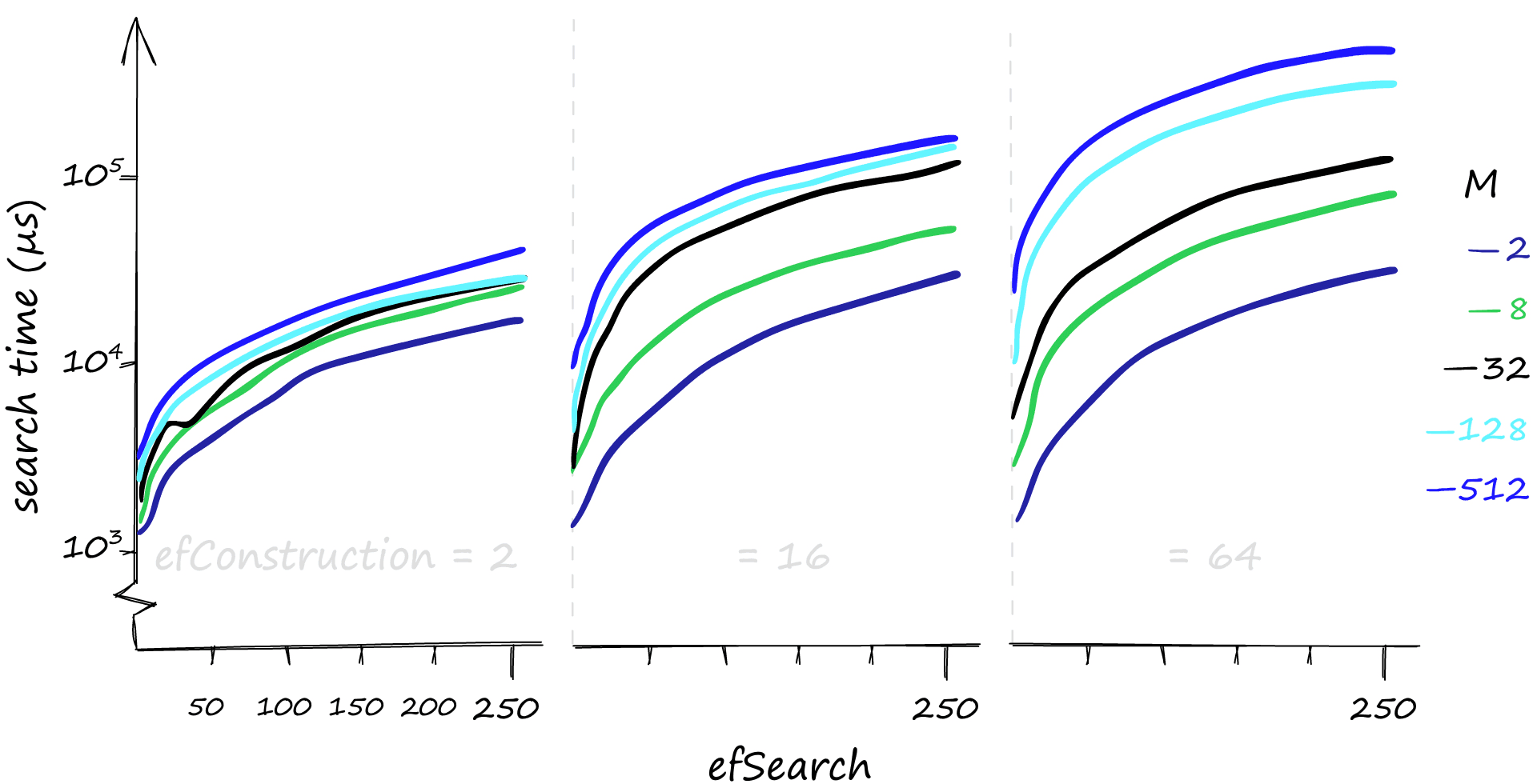
Search time in µs for various M, efConstruction, and efSearch parameters when searching for 1000 queries. Note that the y-axis is using a log scale.
Although higher parameter values provide us with better recall, the effect on search times can be dramatic. Here we search for 1000 similar vectors (xq[:1000]), and our recall/search-time can vary from 80%-1ms to 100%-50ms. If we’re happy with a rather terrible recall, search times can even reach 0.1ms.
If you’ve been following our articles on vector similarity search, you may recall that efConstruction has a negligible effect on search-time — but that is not the case here…
When we search using a few queries, it is true that efConstruction has little effect on search time. But with the 1000 queries used here, the small effect of efConstruction becomes much more significant.
If you believe your queries will mostly be low volume, efConstruction is a great parameter to increase. It can improve recall with little effect on search time, particularly when using lower M values.
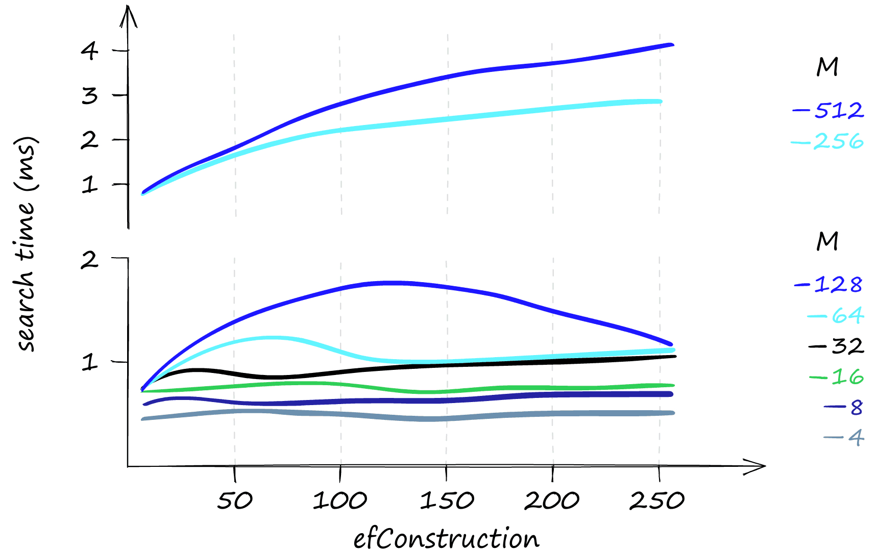
efConstruction and search time when searching for only one query. When using lower M values, the search time remains almost unchanged for different efConstruction values.
That all looks great, but what about the memory usage of the HNSW index? Here things can get slightly less appealing.
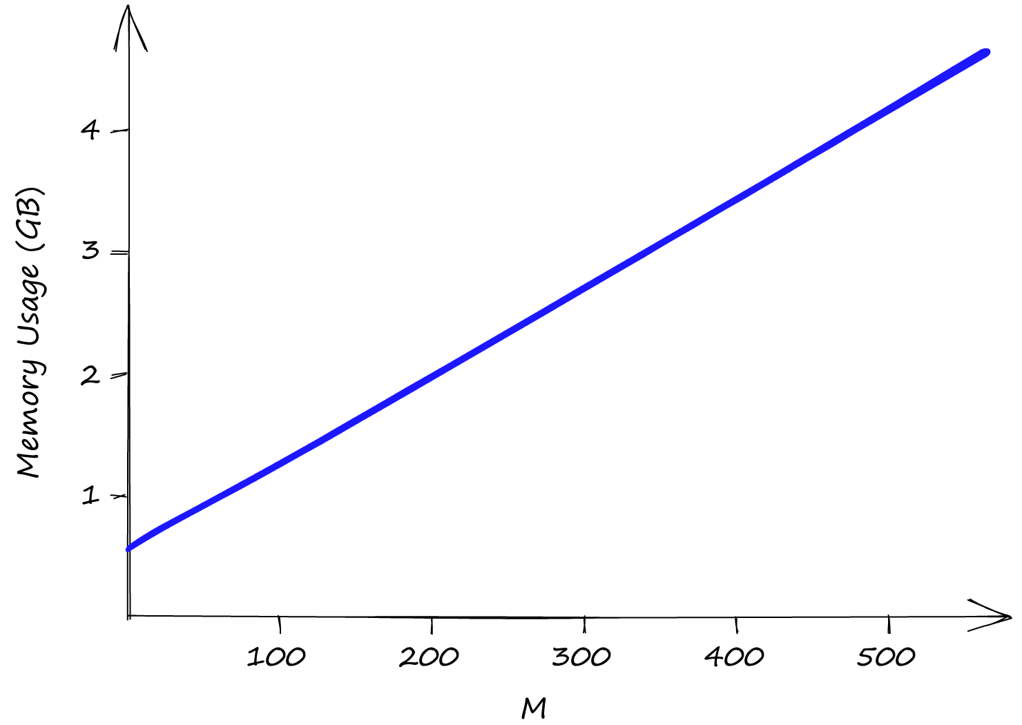
Memory usage with increasing values of M using our Sift1M dataset. efSearch and efConstruction have no effect on the memory usage.
Both efConstruction and efSearch do not affect index memory usage, leaving us only with M. Even with M at a low value of 2, our index size is already above 0.5GB, reaching almost 5GB with an M of 512.
So although HNSW produces incredible performance, we need to weigh that against high memory usage and the inevitable high infrastructure costs that this can produce.
Improving Memory Usage and Search Speeds
HNSW is not the best index in terms of memory utilization. However, if this is important and using another index isn’t an option, we can improve it by compressing our vectors using product quantization (PQ). Using PQ will reduce recall and increase search time — but as always, much of ANN is a case of balancing these three factors.
If, instead, we’d like to improve our search speeds — we can do that too! All we do is add an IVF component to our index. There is plenty to discuss when adding IVF or PQ to our index, so we wrote an entire article on mixing-and-matching of indexes.
That’s it for this article covering the Hierarchical Navigable Small World graph for vector similarity search! Now that you’ve learned the intuition behind HNSW and how to implement it in Faiss, you’re ready to go ahead and test HNSW indexes in your own vector search applications, or use a managed solution like Pinecone or OpenSearch that has vector search ready-to-go!
If you’d like to continue learning more about vector search and how you can use it to supercharge your own applications, we have a whole set of learning materials aiming to bring you up to speed with the world of vector search.
References
[1] E. Bernhardsson, ANN Benchmarks (2021), GitHub
[2] W. Pugh, Skip lists: a probabilistic alternative to balanced trees (1990), Communications of the ACM, vol. 33, no.6, pp. 668-676
[3] Y. Malkov, D. Yashunin, Efficient and robust approximate nearest neighbor search using Hierarchical Navigable Small World graphs (2016), IEEE Transactions on Pattern Analysis and Machine Intelligence
[4] Y. Malkov et al., Approximate Nearest Neighbor Search Small World Approach (2011), International Conference on Information and Communication Technologies & Applications
[5] Y. Malkov et al., Scalable Distributed Algorithm for Approximate Nearest Neighbor Search Problem in High Dimensional General Metric Spaces (2012), Similarity Search and Applications, pp. 132-147
[6] Y. Malkov et al., Approximate nearest neighbor algorithm based on navigable small world graphs (2014), Information Systems, vol. 45, pp. 61-68
[7] M. Boguna et al., Navigability of complex networks (2009), Nature Physics, vol. 5, no. 1, pp. 74-80
[8] Y. Malkov, A. Ponomarenko, Growing homophilic networks are natural navigable small worlds (2015), PloS one
Facebook Research, Faiss HNSW Implementation, GitHub
Was this article helpful?