





Leverage large language models, state-of-the-art text and speech analytics tools, and vector databases to build an end-to-end audio recommendation solution.
Audio streaming services are becoming increasingly popular, and the ability to recommend songs and podcasts to users based on their listening history is becoming increasingly important. However, the abundance of audio content can overwhelm users, so creating an audio recommendation system can help users discover new and relevant content they will enjoy.
This article will explore how to build an audio recommendation system using Python. We begin with a brief overview of recommendation systems before diving into their application in the audio domain through a step-by-step Python tutorial.
Before diving into the technical implementation, let’s look at the general workflow of the recommendation system we are trying to build.
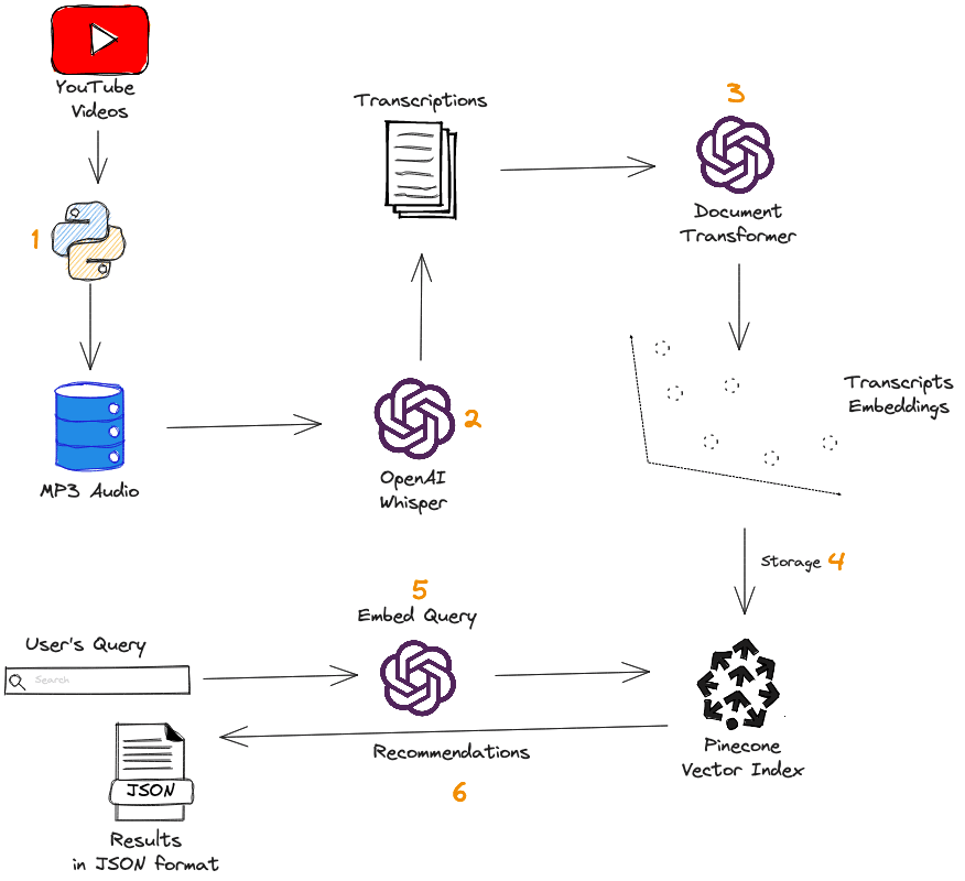
Recommendation workflow and main components
First, we collect YouTube videos and transform each into audio using Python. The OpenAI Whisper model is then used to transcribe audio to text. After that, we use the text-embedding-ada-002 model to generate transcription embeddings. These embeddings are used to populate a Pinecone index, which is used for performing queries.
Whisper models were developed to study the capability of speech-processing systems for speech recognition and translation tasks. They have the ability to transcribe speech audio into text.
OpenAI trained on 680,000 hours of labeled audio data, which the authors report to be one of the largest ever created in supervised speech recognition. Whisper demonstrated considerable resilience and a lower error rate than other models when tested across a broad range of datasets.
To begin, you will need to have Python installed on your computer along with the following libraries:
You can install these libraries using pip like so:
%%bash
pip install pandas
pip install git+https://github.com/openai/whisper.git
pip install pytube
pip install numpy
pip install pinecone-client
Now, let’s import the necessary modules and create the dataset.
# Import the modules
import os
import torch
import whisper
import pinecone
import numpy as np
import pandas as pd
from pytube import YouTubeThe following helper function video_to_audio() first downloads a video from YouTube and saves it as an MP3 audio file. Then it returns the name of the audio file that is later used within the metadata dataframe.
The function takes two main parameters:
def video_to_audio(video_url, destination):

 # Get the video
 video = YouTube(video_url)

 # Convert video to Audio
 audio = video.streams.filter(only_audio=True).first()

 # Save to destination
 output = audio.download(output_path = destination)

 name, ext = os.path.splitext(output)
 new_file = name + '.mp3'

 # Replace spaces with "_"
 new_file = new_file.replace(" ", "_")

 # Change the name of the file
 os.rename(output, new_file)

return new_fileThe dataframe is used to store the metadata and will have the following four main columns:
Before performing these tasks, let’s first create the destination folder.
%%bash
mkdir "audio_data"
# Create URL column
audio_path = "audio_data"
list_videos = ["https://www.youtube.com/watch?v=IdTMDpizis8",
"https://www.youtube.com/watch?v=fLeJJPxua3E",
"https://www.youtube.com/watch?v=z3FA2kALScU",
"https://www.youtube.com/watch?v=yBrRpb8aLwk",
"https://www.youtube.com/watch?v=ERClHCOF14c",
"https://www.youtube.com/watch?v=b-Pn0yXL9y8",
"https://www.youtube.com/watch?v=CYfU9WBy_HA",
"https://www.youtube.com/watch?v=FncTDZxNbM4",
"https://www.youtube.com/watch?v=JjCFoba5hKE",
"https://www.youtube.com/watch?v=YUxR3d10lz4",
"https://www.youtube.com/watch?v=t1XCzWlYWeA",
"https://www.youtube.com/watch?v=RS_HDj2mOkk",
"https://www.youtube.com/watch?v=scvDvVbv1hk", …]
# Create dataframe
transcription_df = pd.DataFrame(list_videos, columns=['URLs'])
transcription_df.head()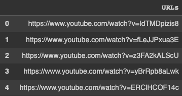
Now, we can create the file_name column using the lambda expression:
transcription_df["file_name"] = transcription_df["URLs"].apply(
    lambda url: video_to_audio(url, audio_path)
)
transcription_df.head()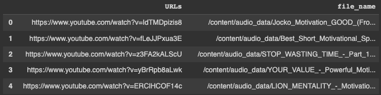
This is the screenshot of the sample of audio files downloaded into the “audio_data” folder after running the previous script.
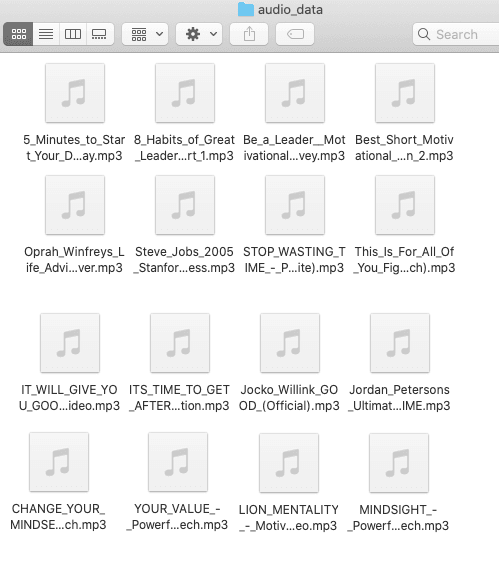
First 16 audio files in the audio_data folder
Before loading the model, it is important to set the device to use GPU when available.
# Set the device
device = "cuda" if torch.cuda.is_available() else "cpu"

# Load the model
whisper_model = whisper.load_model("large", device=device)
The file_name corresponds to the mp3 file in the audio_data folder. Using whisper we can apply a lambda function to generate the transcription of each audio file with the audio_to_text() function.
def audio_to_text(audio_file):
   return whisper_model.transcribe(audio_file)["text"]

# Apply the function to all the audio files
transcription_df["transcriptions"] = transcription_df["file_name"].apply(lambda f_name: audio_to_text(f_name))


# Show the first five rows
transcription_df.head()
We can use the text wrapper of the Python module to format the printing of the text samples as follows:
import textwrap
wrapper = textwrap.TextWrapper(width=60)
first_transcription = transcription_df.iloc[0]["transcriptions"]
formatted_transcription = wrapper.fill(text=first_transcription)
# Check first transcription
print(formatted_transcription)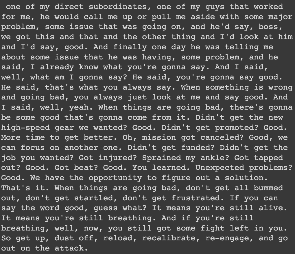
Transcription of the first audio in the document
We can check the total number of documents in the dataframe with the shape function as follows:
display(df_duplicated.shape)
# (147, 3)
There are 147 documents overall and 3 columns.
In this section, we will leverage the text-embedding-ada-002 model from OpenAI to generate the embeddings of the transcriptions.
Even though language models like BERT have been used for multiple use cases, there might be adapted for long-form documents because of the limitations to 512 tokens.
text-embedding-ada-002 is the GPT-3 Ada second-generation model made available by OpenAI through their embedding model API. This model beats all existing embedding models available in the API on almost all tasks while remaining the cheapest option.
Instead of having multiple different models fine-tuned for specific tasks, Ada is capable of handling all tasks, and has shown the following performance in the benchmarking test:
The new architecture introduced in the second generation of Ada led to the increase from 2048 to 8096 tokens, which is adapted when dealing with longer documents or other forms of extended text content.
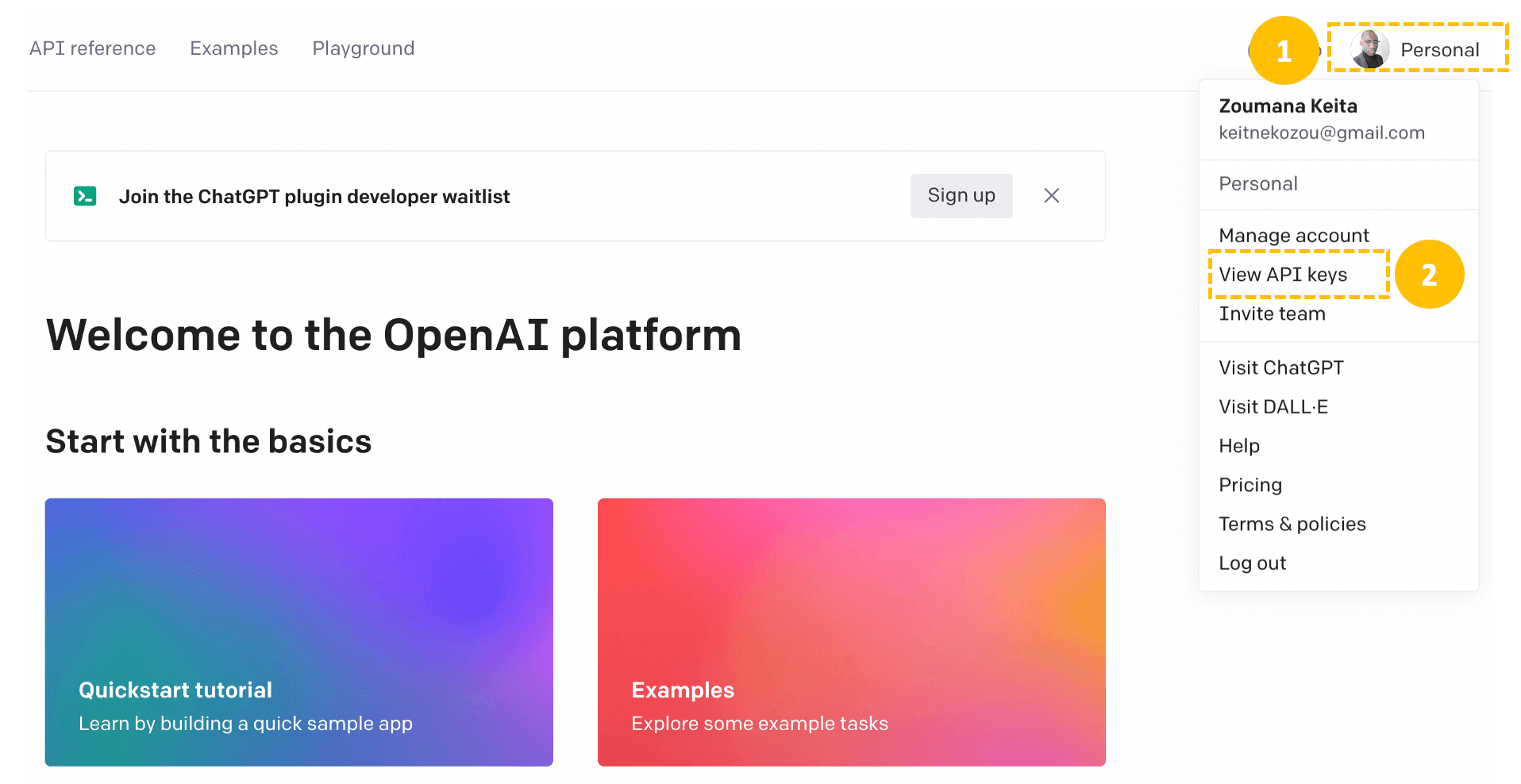
Creating an OpenAI developer account is the first step to accessing the API key to interact with the model, and all the steps are illustrated below once on the official website.
Then, Create a new secret key from the “Create new secret key” tab by providing a meaningful name (OpenAI_API_Key in this case), and then the API key is automatically generated.
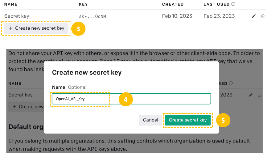
With these credentials, the next steps include: (1) the installation of the OpenAI API, (2) defining the general pattern of the code to interact with the model:
# Install the library
pip install openai

# import openai
import openai

# Set up the OpenAI key
openai.api_key = "<YOUR_API_KEY_HERE>"
The general code pattern for calling the model via the API is given below:
def get_embeddings(text_to_embed):
	response = openai.Embedding.create(
    	model= "text-embedding-ada-002",
    	input=[text_to_embed]
	)
	# Extract the AI output embedding as a list of floats
	embedding = response["data"][0]["embedding"]
return embeddingThis helper function can be applied to generate the embeddings for each row in the previous dataframe using a lambda expression.
transcription_df["embedding"] = transcription_df["transcriptions"].astype(str).apply(get_embeddings)By looking at the first five rows of the dataset, we can see that the new embedding column has been created.
display(transcription_df.head())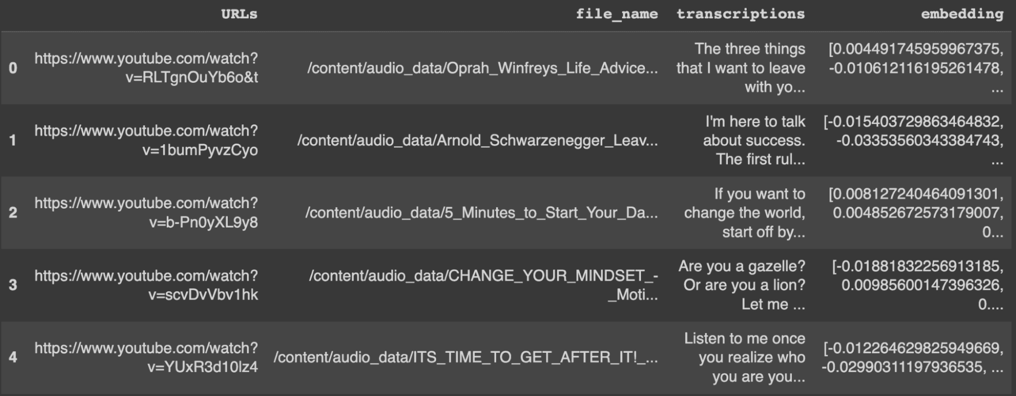
First five rows of the data with the embedding column
We have successfully created a dataframe with all the required information for recommendations. However, these are some of the issues with using dataframes in industry:
Wouldn't it be nice if we could use technology to avoid these issues?
Here is where Pinecone comes in handy.
Pinecone provides a fully-managed, easily scalable vector database that makes it easy to build high-performance vector search applications.
This section illustrates how to configure your Pinecone index and populate it with vector data for building the final recommendation feature.
Before starting, make sure to get your free Pinecone API key.
After getting the API key, the next step is to configure your environment as follows:
import os

# Initialize connection to pinecone
pinecone.init(
  api_key=os.environ.get("PINECONE_API_KEY") or "YOUR_API_KEY",
  environment=os.environ.get("PINECONE_ENVIRONMENT",) or "YOUR_ENV"
)

# Index params
my_index_name = "audio-search"
vector_dim = len(transcription_df.iloc[0].embeddings)

if my_index_name not in pinecone.list_indexes():
  # Create the index
  pinecone.create_index(name = my_index_name,
                      dimension=vector_dim,
                      metric="cosine")
Let’s understand what is happening here.
pinecone.init initializes your Pinecone client using your credentials.audio_search and expected vector dimensionality.Index class.After a successful connection, the following code should show the current state of the vector index.
# Show information about the vector index
my_index.describe_index_stats()
{'dimension': 1536,
'index_fullness': 0.0,
'namespaces': {},
'total_vector_count': 0}We can see that the dimension for each vector is 1536, and total_vector_count is 0, meaning that the index is empty.
With an empty vector index, it is impossible to perform searches. We must populate it with the ID of each video, its URL, the transcriptions, and their embeddings.
transcription_df["vector_id"] = transcription_df.index
transcription_df["vector_id"] = transcription_df["vector_id"].apply(str)

# Get all the metadata
final_metadata = []

for index in range(len(transcription_df)):
final_metadata.append({
    'ID':  index,
    'url': transcription_df_.iloc[index].URLs,
    'transcription': transcription_df_.iloc[index].transcriptions
})

audio_IDs = transcription_df.vector_id.tolist()
audio_embeddings = [arr for arr in transcription_df.embedding]

# Create the single list of dictionary format to insert
data_to_upsert = list(zip(audio_IDs, audio_embeddings, final_metadata))

# Upload the final data
my_index.upsert(vectors = data_to_upsert)

# Show information about the vector index
my_index.describe_index_stats()
After populating the vector index, we see the following stats from the namespace.
{'dimension': 1536,
'index_fullness': 0.0,
'namespaces': {'': {'vector_count': 147}},
'total_vector_count': 147}
We now have 147 vectors in the index, and the same information can be found on the Pinecone index page.
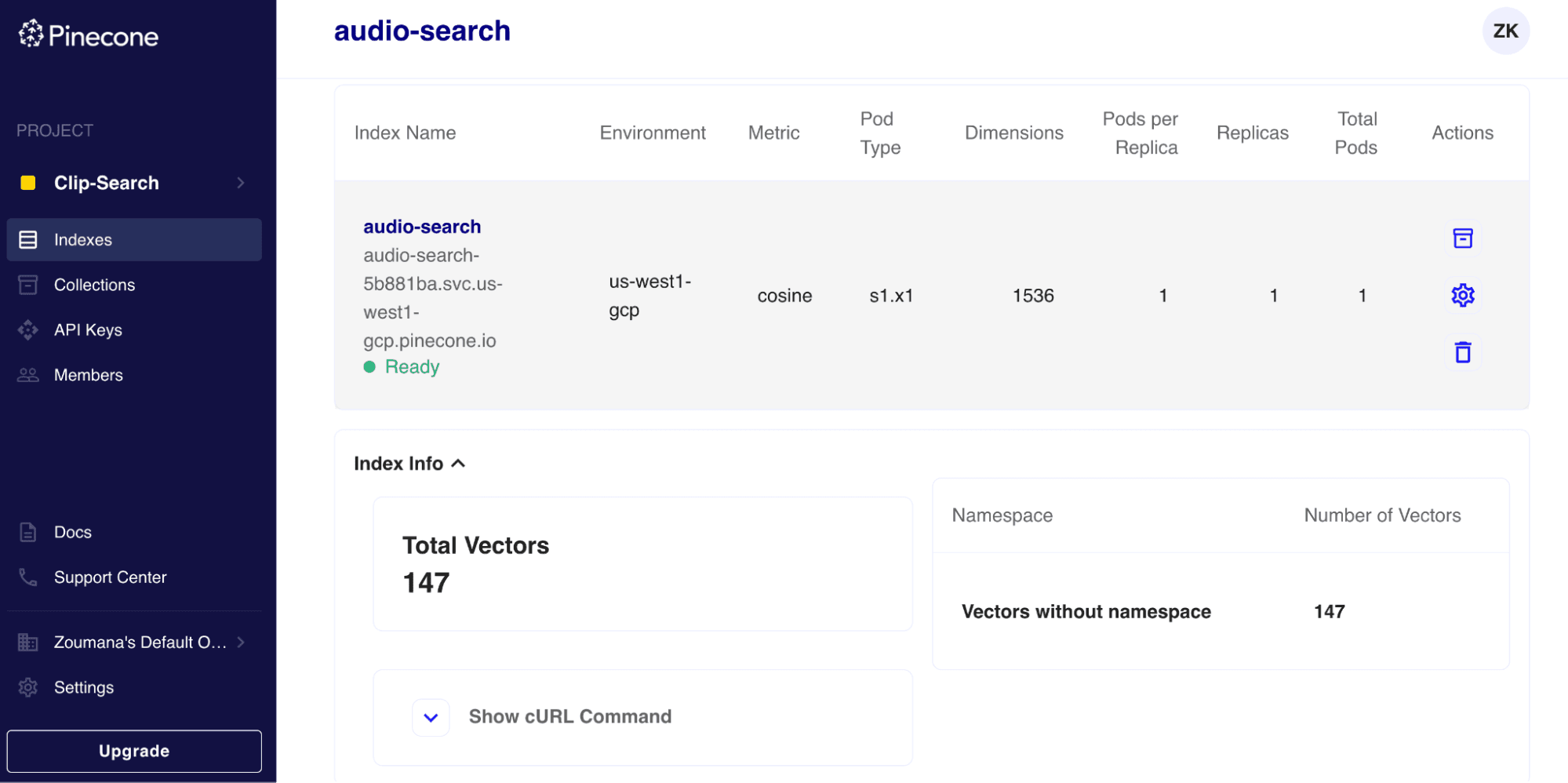
audio-search index details on Pinecone
We can now recommend users similar audio based on input audio. Let’s consider recommending the top 3 audio.
First, we convert the input vector into a list to meet the query format. Then using the query() function, we can recommend the N-1 audio resources along with all the medatada and similarity scores. You can decide not to include the metadata by setting the include_metadata parameter to False.
When interpreting the results, ensure not to include the first index, since it corresponds to the similarity between a vector and itself, which is 100%.
N = 3
my_query_embedding = transcription_df.embedding[0]

# Run the Query Search
my_index.query(my_query_embedding, top_k=N, include_metadata=True)
Below is the final result in JSON format. The output transcription fields have been truncated afterward for a better visualization.
{'matches': [{'id': '0',
          	'metadata': {'ID': 0.0,
                       	'transcription':
                             ' The three things that I want to '
                             'leave with you, just these three, '
                             'I could do ten, I could do a '
                              ...

                             'Phenomenally, phenomenal class of '
                             '2012. Thank you. Thank you. Thank '
                             'you.',
                       	'url': 'https://www.youtube.com/watch?v=RLTgnOuYb6o&t'},
          	'score': 1.00000012,
          	'values': []},

         	{'id': '135',
          	'metadata': {'ID': 135.0,
                       	'transcription': ...
                          'who you are you stop operating in '
                          'desperation you stop saying yes '

                           ...
                           'possessed with the dream. You got '
                           'to be possessed with the dream.',
                       	'url': 'https://www.youtube.com/watch?v=YUxR3d10lz4&t'},

          	'score': 0.869115889,
          	'values': []},

         	{'id': '38',
          	'metadata': {'ID': 38.0,
                       	'transcription':
                             ' Listen to me once you realize '
                                        	...
                             'nobody else sees it. You have to '
                             "feel it when it's not tangible. "
                                        	...,
                       	'url': 'https://www.youtube.com/watch?v=YUxR3d10lz4'},
          	'score': 0.867912114,
          	'values': []}]
 'namespace': ''}
We can check the result from the links of the matches:

Query Video
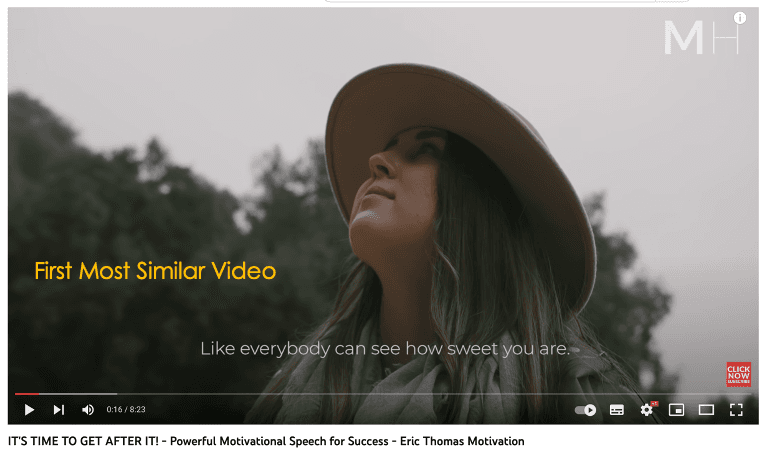
First Most Similar Video with similarity Score = 86.9%
This final JSON format is beneficial and can be used to build any web service application.
Congratulations, you have just learned how to fully implement an audio recommendation solution using state-of-the-art technologies. I hope those technologies' benefits are valid enough to take your project to the next level using vector databases.
Multiple resources are available at our Learning Center to further your learning.
The source code for the article is available on Github.
[1] Alec Radford, Jong Wook Kim, et al., Robust Speech Recognition via Large-Scale Weak Supervision (2022).
[2] Zoumana KEITA, Text-to-Image and Image-to-Image Search Using CLIP (2022)
[3] OpenAI, New and Improved embedding model (2022)
此内容由惯性聚合(RSS阅读器)自动聚合整理,仅供阅读参考。 原文来自 — 版权归原作者所有。