





Over the past several months, people have come to Pinecone after trying and failing with pgvector and other bolt-on vector databases. One common line of thought is: I already have Postgres to store stuff, so why not use it for vector search too? This line of thought seems reasonable at first, but there are much better approaches than this if you want to build a successful Gen AI application.
When we investigated why people choose pgvector initially and then switched to Pinecone, one thing that struck us was how little experimentation went into selecting a database. Instead of evaluating quality first, then simplicity and ease, many users do the opposite. They start using pgvector and other bolt-on solutions out of convenience. But they soon run into complexities and need help to achieve high-quality searches. Thus, they reach out to Pinecone, as the importance of prioritizing quality first, then simplicity becomes evident. They realize that their database needs to provide high search quality to be useful for their Gen AI applications. If they’re tweaking their databases, then that is valuable time they are not spending on building and optimizing their products. And that is detrimental, especially in a fast-moving space like GenAI.
When it comes to vector search, easy is far from simple: vector databases are fundamentally different from traditional databases and document stores, and thinking of vectors as just another type in a Postgres database will not result in a performant solution. Such an attempt defeats the purpose of choosing Postgres in the first place. You will introduce significant complexity even for small and medium workloads for a perceived ease.
Consider one example customer: Notion uses Pinecone to power Notion AI, through which their users continuously create, update, search, and delete vectors in Pinecone. Their users’ usage patterns are highly variable: Some users update their content frequently, others infrequently; some query often, and others only periodically. It is difficult to tune and tweak knobs on pgvector even for predictable, uniform workloads… doing so for highly variable usage patterns across many tenants is nearly impossible.
Moreover, not only does Notion have these strict requirements and large, highly variable workloads, but they also can’t waste time and effort tuning and tweaking knobs, changing resources, and hand-holding their vector database. It would be an expensive operational burden and unrealistic for them.
Postgres is a capable solution for many storage use cases and powers many services and products. But, it is often not the right choice for vector search. In this article, we will examine the architecture of SQL databases like Postgres, how they have bolted-on vector search on top of their core architecture, and why it adds significant operational overheads even for small to medium workloads. We will contrast it with how Pinecone makes it easy to scale vector search by providing low-cost ramp-up, an intuitive UX, and high-quality results with zero hand-holding. Pinecone is purpose-built for powerful vector search, which means that it scales with your workloads seamlessly for a fraction of the cost of other bolt-on solutions, which is why customers like Notion choose Pinecone.
PostgreSQL is a mature and feature-rich Open-Source SQL database, in wide use. It has a powerful extensions API which allows additional functionality to be added to it. One such extension is pgvector, which introduces a new data type and module (vector) and allows users to query this data type, and build vector indexes.
The vector indexes themselves are one of two types:
During writes (to either type of index), pgvector maintains a working set of the index in memory. The working set memory is controlled by the parameter: maintenance_work_mem
We went through a series of various experiments on pgvector to see how the architectural limitations of Postgres have a practical impact on vector workloads. Below, we will go through our findings from a series of experiments on Postgres, using the following four datasets (available via Pinecone Public Datasets):
Let’s start with the first thing one must do for a vector search workload: build an index. Using the Cohere-768 dataset (10 million 768-dimensional vectors), we provisioned a 64 GB RAM VM (more than the total index size), and then, with various subsets of vector counts, we measure the amount of RAM actually used when building the HNSW index:
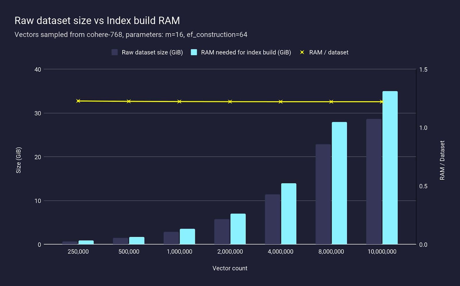
We see that the amount of RAM needed to build an index scales as the dataset does. For Cohere-768, we consistently need RAM proportional to the dataset size, specifically 1.2x of the entire dataset to build the index.
We only found this relationship after over-provisioning the RAM needed for this dataset, which we also knew the exact size of. What happens if you don’t know the exact size of the workload beforehand, as with most production workloads? And even if you do, what happens if you don’t want to massively overprovision the amount of RAM you need for pgvector?
For this modest dataset (28.6GiB) the required amount of RAM (35 GiB) is readily available on typical instances, but for a dataset 2x, 4x or 10x larger, provisioning such instances becomes very costly. Compare this to Pinecone Serverless, where the resources needed to build the index are not the user’s concern — you pay only for the writes to upsert the data and the total space used.
Note that pgvector can page out to disk if RAM is exceeded, which suggests we don’t necessarily have to scale our machines’ RAM as dataset size increases. However, in practical terms, the impact on index build time is significant. Here we re-run the same experiment as above, but with Postgres running on a smaller machine, with the amount of memory available for index build (maintenance_work_mem) set to 16GB. We measure the time taken to index the different dataset sizes:
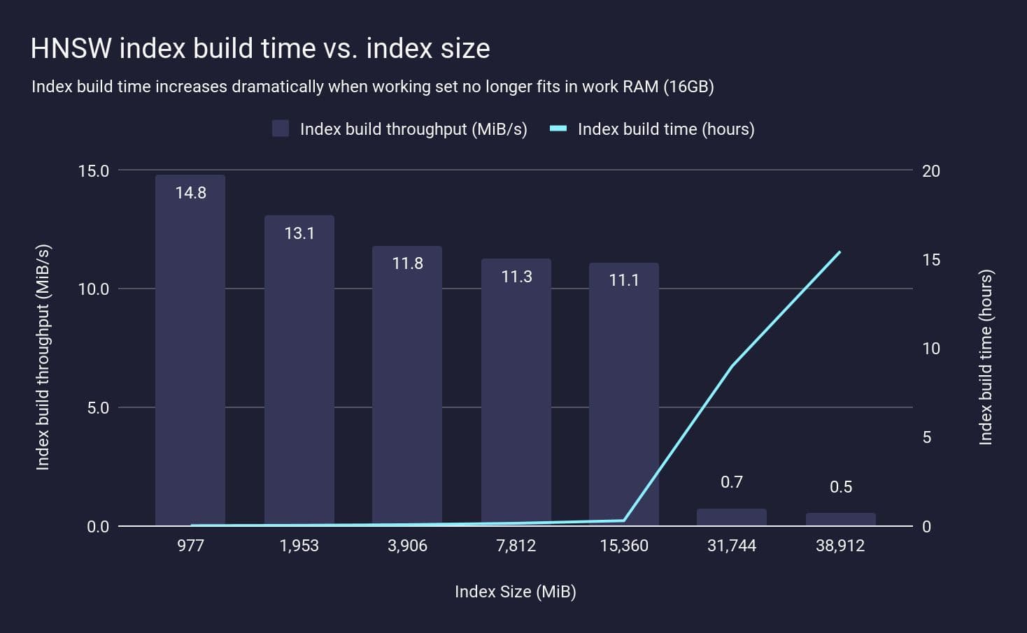
When the HNSW index can fit entirely in RAM (<16GB) we see reasonably constant index build throughput around 10 MiB/s, however once the index exceeds RAM the build throughput drops precipitously — over 10x slower. This is because the HNSW graph has exceeded the working memory, and needs to spill to disk to continue to build the index. As such it’s not feasible to rely on Postgres’s ability to page from disk during index builds and maintain quick build times.
Similar behavior is seen when incrementally updating an existing index. As long as the graph can fit into memory, updates are relatively fast as they don’t require waiting for disk. But, if the index starts exceeding the working set memory, then parts of the index need to be read back from disk before they are modified, and update rate drops by an order of magnitude.
The consequence of this is often an unexpected performance drop when the dataset grows past this critical point. That is, you could build an application with pgvector and achieve your target query latency, then gradually add more data, and when the index no longer fits in RAM and query latency suddenly increases by 10x. Postgres + pgvector does not seem so simple anymore: now you need to start resizing your resources, and in some cases even sharding your database, since you might not have enough RAM to allocate to hold the entire dataset.
Pinecone avoids these problems. With a Serverless index you can simply keep on adding more and more data and query latency stays fast; there’s no index RAM sizing to worry about.
We explored the memory needed for different sized samples of the same dataset (Cohere-768) above, but what about different datasets? Given the importance of ensuring the index fits in RAM, how does one accurately predict how much RAM will be required to build the index for a given workload?
Here we measure the index RAM / dataset ratio to build an index for 4 different datasets — mnist, nq-768-tasb, yfcc and cohere — how much actual RAM is needed to represent the index compared to the input dataset size:
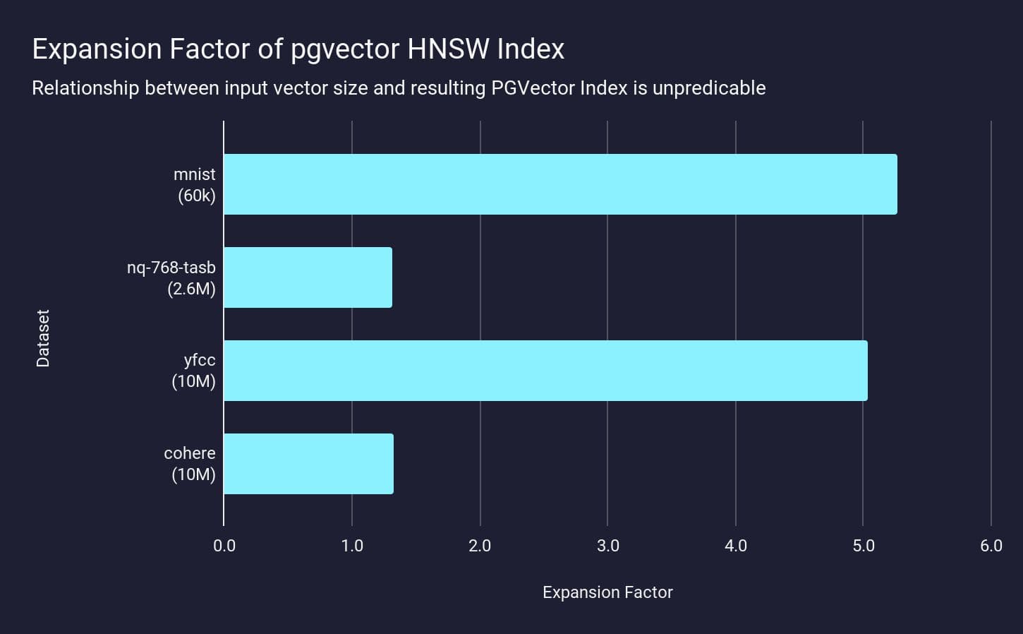
The “expansion factor” — the ratio of the index RAM to the original dataset — varies significantly across the different datasets. The largest expansion is for mnist and yfcc; where the index is over 5x larger than the raw data.
This is counterintuitive: there is no simple way to figure out how to size the index’s working set memory, and the consequences of getting this wrong are significant.
We are just talking about small datasets here. In comparison, Pinecone routinely handles billion scale datasets without customers even having to think about them.
This presents another sizing dimension when using pgvector: you cannot easily predict the size of the vector index (and hence the amount of RAM to be provisioned) without analyzing the dataset itself.
Pinecone serverless avoids this concern; you can upload and query datasets of any size, without having to think about node sizes or counts. You’re just charged based on the amount of data stored.
We also explored an experiment with another common use case in vector databases: metadata filtering.
Metadata filtering is a powerful technique to improve the relevance of vector search by specifying additional predicates to match the queried vectors against. In this experiment, we again use the yfcc-10mm dataset, which consists of images which have been embedded with the CLIP model; along with a “bag” of tags extracted from the description, camera model, year of capture and country. A search is performed specifying an image embedding, plus one or two tags to constrain the search space. Our objective is to achieve high quality recall (≥ 80%) with latency suitable for a real-time application — 200ms or lower, which is realistic for many production applications.
After loading yfcc-10mm, we started trying to submit some queries. At a basic level, PostgreSQL + pgvector supports metadata filtering as a simple WHERE clause added to the SELECT statement. However, this is only post-filtering, meaning the results are filtered after the search occurs. For all practical purposes, this is unusable, since there’s no guarantee about the number of results that are returned. For example, if we just examine the 3rd query from the queries set, zero results are returned instead of the desired 10:
SELECT id, embedding FROM yfcc_10m WHERE metadata @> '{"tags": ["108757"]}' ORDER BY embedding <-> '[...]' LIMIT 10;
...
(0 rows)
If we use EXPLAIN ANALYZE against the query, we can see how the query planner has constructed the query to help us understand the behavior we are seeing:
EXPLAIN ANALYZE SELECT id, embedding FROM yfcc_10m WHERE metadata @> '{"tags": ["108757"]}' ORDER BY embedding <-> '[...]' LIMIT 10;

Limit  (cost=64.84..3298.63 rows=10 width=791) (actual time=1.111..1.111 rows=0 loops=1)
   ->  Index Scan using yfcc_10m_embedding_idx on yfcc_10m  (cost=64.84..32337942.84 rows=100000 width=791) (actual time=1.110..1.110 rows=0 loops=1)
         Order By: (embedding <-> '[...]'::vector)
         Filter: ((metadata -> 'tags'::text) @> '"108757"'::jsonb)
         Rows Removed by Filter: 41
 Planning Time: 0.075 ms
 Execution Time: 1.130 ms
Reading from bottom to top, we see Postgres first performs an Index Scan using the HNSW index (yfcc_10m_embedding_idx), then filters by the specified predicate; however, that discards all rows as none matched.
Increasing the candidates search count (hnsw.ef_search) from the default (40) to the maximum value (1000) manages to increase the number of found records from 0 to 1, but 9 of the requested 10 are still not returned.
This is a known issue with pgvector — see pgvector issue #263 and issue #259. The crux of these issues is that pgvector’s HNSW implementation does not have support for metadata filtering as part of the index itself. While one can build partitioned HNSW indexes, this isn’t practical when the cardinality of the predicate being used is high. In the case of yfcc-10mm, there are over 200,000 possible tags, so we would need to build and maintain 200,000 indexes if partitioning was utilized!
What we want is pre-filtering, meaning the corpus is filtered first and then the search occurs, returning the top_k nearest neighbors that match the filter. This is the only way to guarantee that we actually get top_k results every time.
Postgres offers another solution for this problem. For this kind of highly selective query, there is another index type provided: Generalized Inverted Index (GIN). This index type can be used to index semi-structured data like the sets of tags we have here, allowing Postgres to efficiently identify matching documents first (i.e. pre-filtering), and then calculating vector distances of the (hopefully small) remaining candidates.
So, we create a GIN index on the metadata field via:
postgres=# CREATE INDEX ON yfcc_10M USING gin (metadata);The addition of the GIN index does improve results for some queries - the above query now uses the metadata index first; then performs an exhaustive kNN search on the matching rows. This results in recall increasing from 0% of 100%, with a query latency of 3.3ms; still well within our 200ms requirement:
EXPLAIN ANALYZE SELECT id, embedding FROM yfcc_10m WHERE metadata @> '{"tags": ["108757"]}' ORDER BY embedding <-> '[...]' LIMIT 10;

 Limit  (cost=3718.63..3718.66 rows=10 width=791) (actual time=3.232..3.235 rows=10 loops=1)
   ->  Sort  (cost=3718.63..3720.95 rows=929 width=791) (actual time=3.231..3.232 rows=10 loops=1)
         Sort Key: ((embedding <-> '[...]'::vector))
         Sort Method: top-N heapsort  Memory: 42kB
         ->  Bitmap Heap Scan on yfcc_10m  (cost=43.44..3698.56 rows=929 width=791) (actual time=2.892..3.187 rows=148 loops=1)
               Recheck Cond: (metadata @> '{"tags": ["108757"]}'::jsonb)
               Heap Blocks: exact=138
               ->  Bitmap Index Scan on yfcc_10m_metadata_idx  (cost=0.00..43.20 rows=929 width=0) (actual time=2.868..2.868 rows=148 loops=1)
                     Index Cond: (metadata @> '{"tags": ["108757"]}'::jsonb)
 Planning Time: 0.172 ms
 Execution Time: 3.258 ms
(11 rows)
We see here that the pre-filtering via the metadata index (Bitmap Index Scan) identified the 148 rows which matched the predicate in 3.187ms, calculating the distance to those small number of vectors and sorting the top 10 is fast, taking 0.05ms.
However, this isn’t the case for all queries. For example another query, while appearing similar, only results in a recall of 50% because the GIN metadata index was not consulted and only the HNSW index was used:
SELECT id, embedding FROM yfcc_10M WHERE metadata @> '{"tags": ["1225"]}' ORDER BY embedding <-> '[135.0, 82.0, 151.0, ..., 126.0]' LIMIT 10;
...
(5 rows)
EXPLAIN ANALYZE SELECT id, embedding FROM yfcc_10M WHERE metadata @> '{"tags": ["1225"]}' ORDER BY embedding <-> '[...]' LIMIT 10;
QUERY PLAN
Limit (cost=64.84..3508.90 rows=10 width=791) (actual time=14.743..15.452 rows=5 loops=1)
-> Index Scan using yfcc_10m_embedding_idx on yfcc_10m (cost=64.84..32312927.39 rows=93822 width=791) (actual time=14.742..15.449 rows=5 loops=1)
Order By: (embedding <-> '[...]'::vector)
Filter: (metadata @> '{"tags": ["1225"]}'::jsonb)
Rows Removed by Filter: 1044
Planning Time: 0.174 ms
Execution Time: 15.474 ms
(7 rows)In another instance, the query planner didn’t use the HNSW index at all, resulting in a very slow (3.8s) query due to it performing a full table scan (“Parallel Seq Scan”):
EXPLAIN ANALYZE SELECT id, embedding FROM yfcc_10M WHERE metadata @> '{"tags": ["3432"]}' AND metadata @> '{"tags": ["3075"]}' ORDER BY embedding <-> '[...]' LIMIT 10;

QUERY PLAN

 Limit  (cost=1352639.11..1352639.12 rows=1 width=791) (actual time=3786.265..3792.470 rows=10 loops=1)
   ->  Sort  (cost=1352639.11..1352639.12 rows=1 width=791) (actual time=3730.084..3736.288 rows=10 loops=1)
         Sort Key: ((embedding <-> '[...]'::vector))
         Sort Method: top-N heapsort  Memory: 43kB
         ->  Gather  (cost=1000.00..1352639.10 rows=1 width=791) (actual time=4.756..3734.891 rows=2259 loops=1)
               Workers Planned: 2
               Workers Launched: 2
               ->  Parallel Seq Scan on yfcc_10m  (cost=0.00..1351639.00 rows=1 width=791) (actual time=113.590..3711.979 rows=753 loops=3)
                     Filter: ((metadata @> '{"tags": ["3432"]}'::jsonb) AND (metadata @> '{"tags": ["3075"]}'::jsonb))
                     Rows Removed by Filter: 3332580
 Planning Time: 0.250 ms
 Execution Time: 3792.897 ms
(16 rows)

Time: 3793.678 ms (00:03.794)
It’s not clear why the query planner decides to use or not use a particular index, and the choice can vary across what appear to be similar queries. In short: Getting consistent, high quality results with low latency can require extensive tuning of the database and its indexes. And even then, it might not be possible. With Pinecone, you can expect high quality results with a small fraction of the latency without any tuning.
Our initial objective was 200ms latency and at least 80% p95 recall. Note that pgvector cannot achieve this object for even half of the queries (p50), let alone the vast majority of queries (p95):
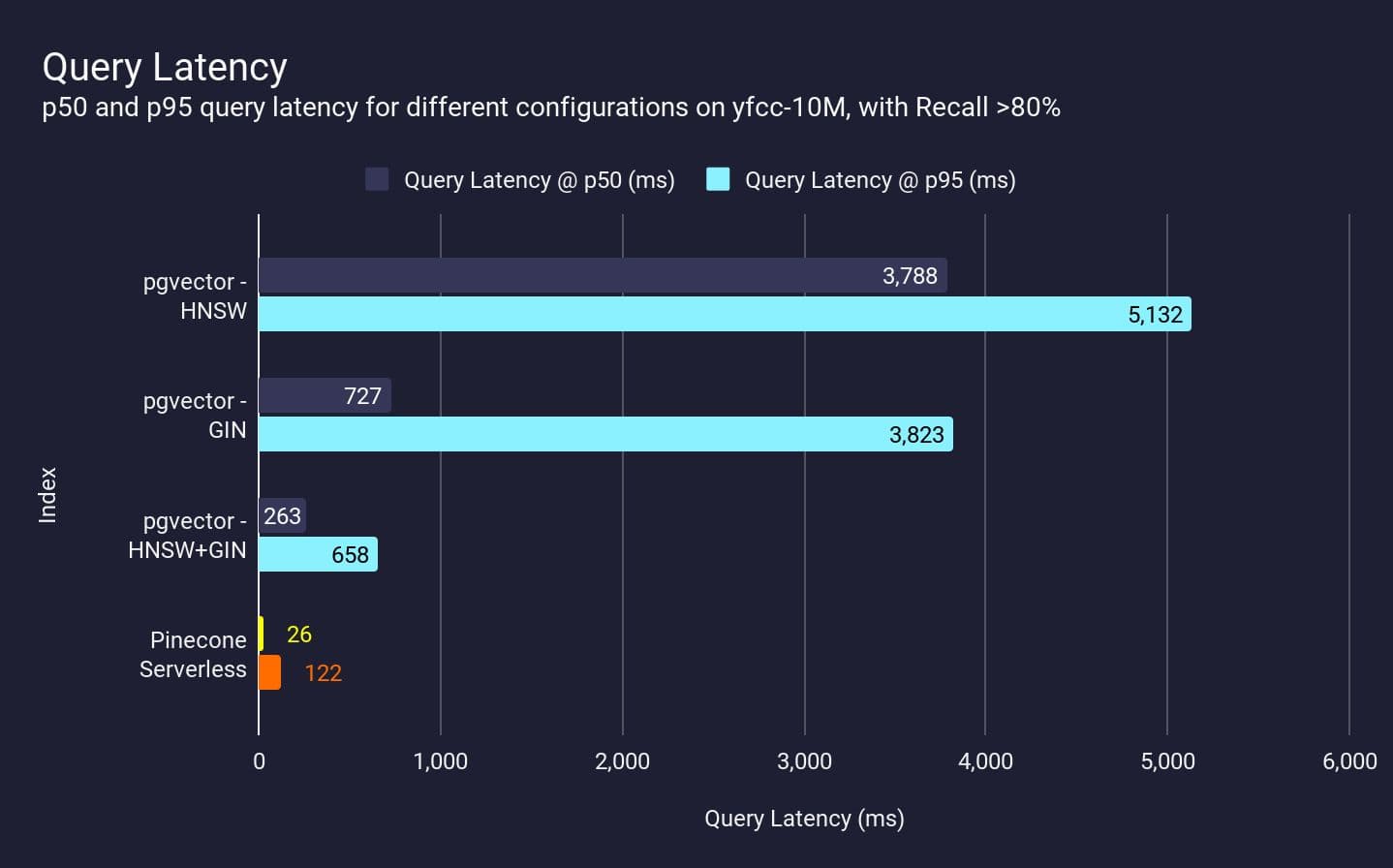
In comparison, Pinecone Serverless achieves this target with zero tuning at both p50 and p95, out of the box. For any non-trivial workload that requires filtering, it’s impractical to rely on Postgres, regardless of the tuning and setup.
We mentioned earlier that pgvector offers another type of index: IVF-Flat. This is appealing because the memory requirements are often much lower than HNSW, sometimes as low as 1/10th. However, because of its architecture, IVF-Flat doesn’t handle “drift” well. That is, changes or updates after the index is initially built will become problematic for IVF-Flat indexes.
Consider two basic workloads:
For each workload, we built the IVF-Flat index with the recommended configuration (lists = rows / 1000 for up to 1M rows and sqrt(rows) for over 1M rows). Query parameter (ivfflat.probes) is set to the largest value which results in p95 query latency under 100ms. We then measured the recall of the baseline workload vs the drift workload):
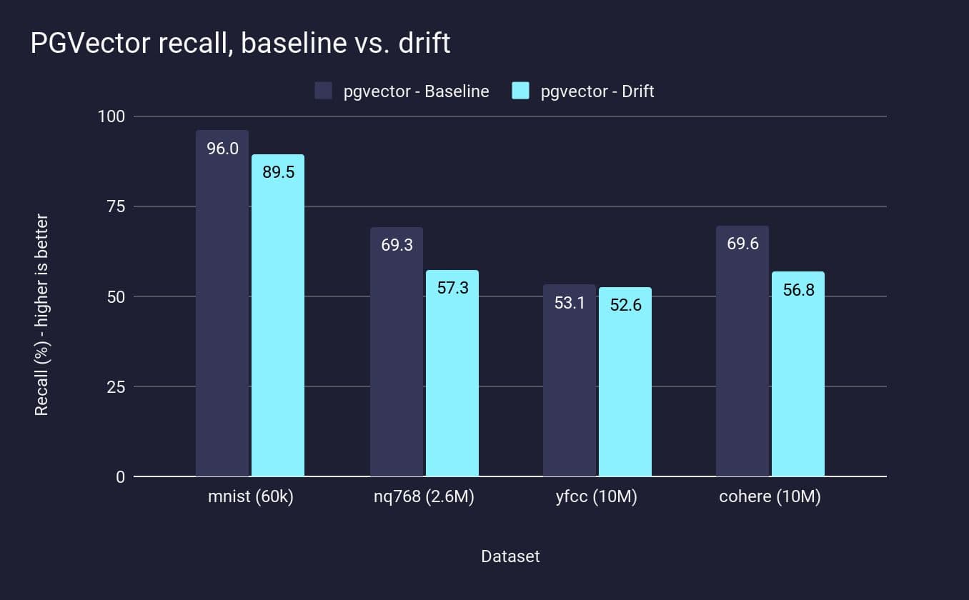
We can see that across the datasets, pgvector’s recall drops when the dataset has drifted since the initial IVF-Flat partitions were created. In a practical sense, this means that, unless you have the exact data you want to upload, and you never update that data, IVF-Flat indexes will not be able to support your application. In fact, even if you do have all the data and never update it, your recall will still not be as high in Postgres as in Pinecone:
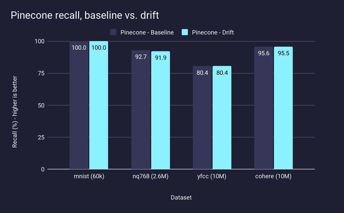
For Pinecone Serverless, we get high recall to begin with, and even after drift, we maintain that high recall. It’s not realistic to expect that customers have static data, which is why we built Pinecone to support these use cases.
We’ve looked at various metrics relating to quality, since the goal of this post was the focus on experience and the architectural limitations of using Postgres, as well as how we built Pinecone to mitigate these headaches and solve the bottlenecks. At the same time, though, we also want to offer an affordable solution with pay-as-you-go pricing that scales for customers as they grow. So: what are the basic cost comparisons of these various workloads? Here we model the cost per month to perform a given workload pattern on each dataset:
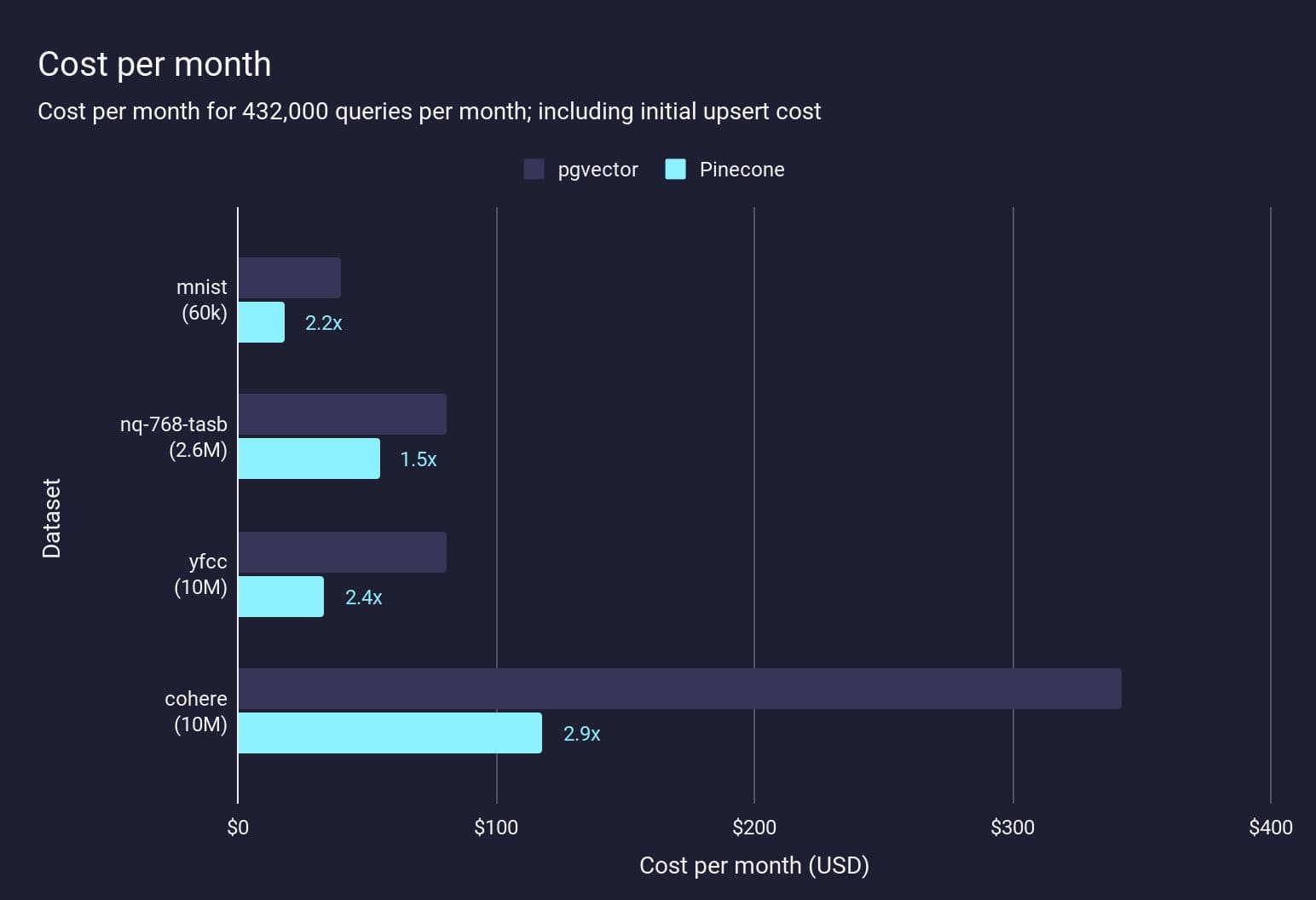
For Pinecone, the cost is estimated using the Pinecone's cost estimator, for pgvector it is the monthly cost of the EC2 instance needed to run the workload at <100ms p95 query latency, plus the EBS cost.
Costs will vary for different workloads, but here we see that Pinecone Serverless is cheaper for the four tested datasets — even including the one-off initial upsert cost — by a factor of 1.1x–2.2x. If we only consider the ongoing monthly cost then the cost difference is even more significant: between 1.5x and 2.9x lower. These are, in fact, relatively small workloads for the scale that Pinecone can handle.
This doesn’t even include the cost of maintaining the Postgres database, high availability and other aspects of managed databases that dramatically reduce the overhead of maintaining and operating these databases — all of which is provided out of the box by Pinecone.
We understand that all workloads look different, so we encourage you to test out Pinecone for yourself.
此内容由惯性聚合(RSS阅读器)自动聚合整理,仅供阅读参考。 原文来自 — 版权归原作者所有。