Dense Vectors: Capturing Meaning with Code

Pinecone is a vector database for storing and searching through dense vectors. Why would you ever want to do that? Keep reading to find out, then try Pinecone for free.

There is perhaps no greater contributor to the success of modern Natural Language Processing (NLP) technology than vector representations of language. The meteoric rise of NLP was ignited with the introduction of word2vec in 2013 [1].

Word2vec is one of the most iconic and earliest examples of dense vectors representing text. But since the days of word2vec, developments in representing language have advanced at ludicrous speeds.

This article will explore why we use dense vectors — and some of the best approaches to building dense vectors available today.

Dense vs Sparse Vectors

The first question we should ask is why should we represent text using vectors? The straightforward answer is that for a computer to understand human-readable text, we need to convert our text into a machine-readable format.

Language is inherently full of information, so we need a reasonably large amount of data to represent even small amounts of text. Vectors are naturally good candidates for this format.

We also have two options for vector representation; sparse vectors or dense vectors.

Sparse vectors can be stored more efficiently and allow us to perform syntax-based comparisons of two sequences. For example, given two sentences; "Bill ran from the giraffe toward the dolphin", and "Bill ran from the dolphin toward the giraffe" we would get a perfect (or near-perfect) match.

Why? Because despite the meaning of the sentences being different, they are composed of the same syntax (e.g., words). And so, sparse vectors would be closely or even perfectly matched (depending on the construction approach).

Where sparse vectors represent text syntax, we could view dense vectors as numerical representations of semantic meaning. Typically, we are taking words and encoding them into very dense, high-dimensional vectors. The abstract meaning and relationship of words are numerically encoded.

Sparse vectors are called sparse because vectors are sparsely populated with information. Typically we would be looking at thousands of zeros to find a few ones (our relevant information). Consequently, these vectors can contain many dimensions, often in the tens of thousands.

clustered

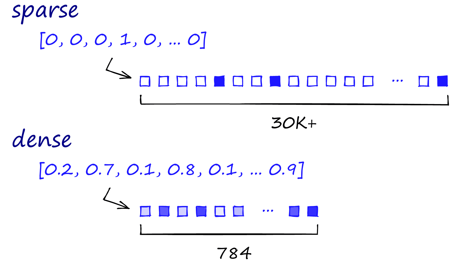
Sparse and dense vector comparison. Sparse vectors contain sparsely distributed bits of information, whereas dense vectors are much more information-rich with densely-packed information in every dimension.

Dense vectors are still highly dimensional (784-dimensions are common, but it can be more or less). However, each dimension contains relevant information, determined by a neural net — compressing these vectors is more complex, so they typically use more memory.

Imagine we create dense vectors for every word in a book, reduce the dimensionality of those vectors and then visualize them in 3D — we will be able to identify relationships. For example, days of the week may be clustered together:

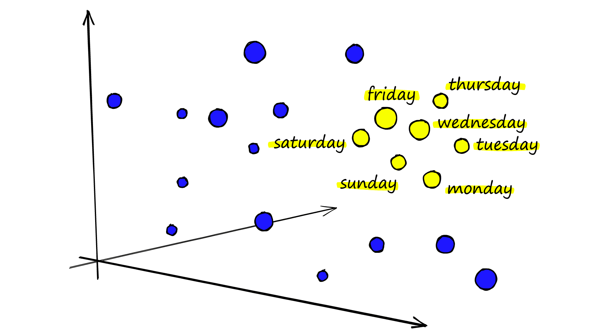
Example of the clustering of related keywords as is typical with word embeddings such as word2vec or GLoVe.

Or we could perform ‘word-based’ arithmetic:

A classic example of arithmetic performed on word vectors from another Mikolov paper [2].

And all of this is achieved using equally complex neural nets, which identify patterns from massive amounts of text data and translate them into dense vectors.

Therefore we can view the difference between sparse and dense vectors as representing syntax in language versus representing semantics in language.

Generating Dense Vectors

Many technologies exist for building dense vectors, ranging from vector representations of words or sentences, Major League Baseball players [3], or even cross-media text and images.

We usually take an existing public model to generate vectors. For almost every scenario there is a high-performance model out there and it is easier, faster, and often much more accurate to use them. There are cases, for example for industry or language-specific embeddings where you sometimes need to fine-tune or even train a new model from scratch, but it isn’t common.

We will explore a few of the most exciting and valuable of these technologies, including:

The ‘2vec’ methods
Sentence Transformers
Dense Passage Retrievers (DPR)
Vision Transformers (ViT)

Word2Vec

Although we now have superior technologies for building embeddings, no overview on dense vectors would be complete without word2vec. Although not the first, it was the first widely used dense embedding model thanks to (1) being very good, and (2) the release of the word2vec toolkit — allowing easy training or usage of pre-trained word2vec embeddings.

Given a sentence, word embeddings are created by taking a specific word (translated to a one-hot encoded vector) and mapping it to surrounding words through an encoder-decoder neural net.

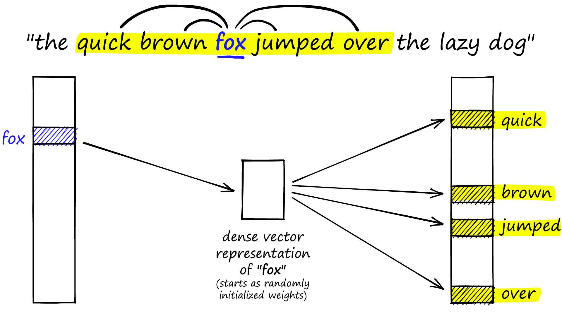
The skip-gram approach to building dense vectors embeddings in word2vec.

This is the skip-gram version of word2vec which, given a word fox, attempts to predict surrounding words (its context). After training we discard the left and right blocks, keeping only the middle dense vector. This vector represents the word to the left of the diagram and can be used to embed this word for downstream language models.

We also have the continuous bag of words (CBOW), which switches the direction and aims to predict a word based on its context. This time we produce an embedding for the word on the right (in this case, still fox).

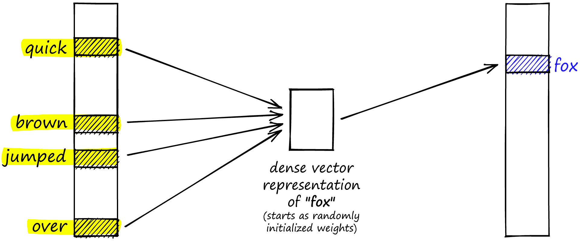
The continuous bag of words (CBOW) approach to building dense vector embeddings in word2vec.

Both skip-gram and CBOW are alike in that they produce a dense embedding vector from the middle hidden layer of the encoder-decoder network.

From this, Mikolov et al. produced the infamous King - Man + Woman == Queen example of vector arithmetic applied to language we saw earlier [2].

Word2vec spurred a flurry of advances in NLP. Still, when it came to representing longer chunks of text using single vectors — word2vec was useless. It allowed us to encode single words (or n-grams) but nothing more, meaning long chunks of text could only be represented by many vectors.

To compare longer chunks of text effectively we need it to be represented by a single vector. Because of this limitation, several extended embedding methods quickly cropped up, such as sentence2vec and doc2vec.

Whether word2vec, sentence2vec, or even (batter|pitcher)2vec (representations of Major League Baseball players [3]), we now have vastly superior technologies for building these dense vectors. So although ‘2vec’ is where it started, we don’t often see them in use today.

Sentence Similarity

We’ve explored the beginnings of word-based embedding with word2vec and briefly touched on the other 2vecs that popped up, aiming to apply this vector embedding approach to longer chunks of text.

We see this same evolution with transformer models. These models produce incredibly information-rich dense vectors, which can be used for a variety of applications from sentiment analysis to question-answering. Thanks to these rich embeddings, transformers have become the dominant modern-day language models.

BERT is perhaps the most famous of these transformer architectures (although the following applies to most transformer models).

Within BERT, we produce vector embeddings for each word (or token) similar to word2vec. However, embeddings are much richer thanks to much deeper networks — and we can even encode the context of words thanks to the attention mechanism.

The attention mechanism allows BERT to prioritize which context words should have the biggest impact on a specific embedding by considering the alignment of said context words (we can imagine it as BERT literally paying attention to specific words depending on the context).

What we mean by ‘context’ is, where word2vec would produce the same vector for ‘bank’ whether it was “a grassy bank” or “the bank of England” — BERT would instead modify the encoding for bank based on the surrounding context, thanks to the attention mechanism.

However, there is a problem here. We want to focus on comparing sentences, not words. And BERT embeddings are produced for each token. So this doesn’t help us in sentence-pair comparisons. What we need is a single vector that represents our sentences or paragraphs like sentence2vec.

The first transformer explicitly built for this was Sentence-BERT (SBERT), a modified version of BERT [4].

BERT (and SBERT) use a WordPiece tokenizer — meaning that every word is equal to one or more tokens. SBERT allows us to create a single vector embedding for sequences containing no more than 128 tokens. Anything beyond this limit is cut.

This limit isn’t ideal for long pieces of text, but more than enough when comparing sentences or small-average length paragraphs. And many of the latest models allow for longer sequence lengths too!

Embedding With Sentence Transformers

Let’s look at how we can quickly pull together some sentence embeddings using the sentence-transformers library [5]. First, we import the library and initialize a sentence transformer model from Microsoft called all-mpnet-base-v2 (maximum sequence length of 384).

```bash
!pip install sentence-transformers
```

In[1]:

from sentence_transformers import SentenceTransformer

model = SentenceTransformer('all-mpnet-base-v2')

Out[1]:

Downloading: 100%|██████████| 1.18k/1.18k [00:00<00:00, 314kB/s]
Downloading: 100%|██████████| 10.1k/10.1k [00:00<00:00, 2.61MB/s]
Downloading: 100%|██████████| 571/571 [00:00<00:00, 200kB/s]
...
Downloading: 100%|██████████| 190/190 [00:00<00:00, 46.5kB/s]

And what does our sentence transformer produce from these sentences? A 768-dimensional dense representation of our sentence. The performance of these embeddings when compared using a similarity metric such as cosine similarity is, in most cases — excellent.

In[2]:

sentences = [
    "it caught him off guard that space smelled of seared steak",
    "she could not decide between painting her teeth or brushing her nails",
    "he thought there'd be sufficient time is he hid his watch",
    "the bees decided to have a mutiny against their queen",
    "the sign said there was road work ahead so she decided to speed up",
    "on a scale of one to ten, what's your favorite flavor of color?",
    "flying stinging insects rebelled in opposition to the matriarch"
]

In[3]:

embeddings = model.encode(sentences)
embeddings.shape

Despite our most semantically similar sentences about bees and their queen sharing zero descriptive words, our model correctly embeds these sentences in the closest vector space when measured with cosine similarity!

Question-Answering

Another widespread use of transformer models is for questions and answers (Q&A). Within Q&A, there are several different architectures we can use. One of the most common is open domain Q&A (ODQA).

ODQA allows us to take a big set of sentences/paragraphs that contain answers to our questions (such as paragraphs from Wikipedia pages). We then ask a question to return a small chunk of one (or more) of those paragraphs which best answers our question.

When doing this, we are making use of three components or models:

Some sort of database to store our sentence/paragraphs (called contexts).
A retriever retrieves contexts that it sees as similar to our question.
A reader model which extracts the answer from our related context(s).

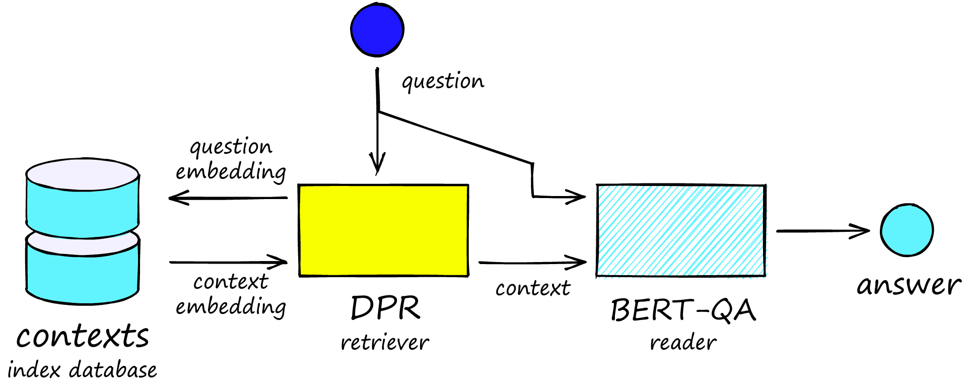
An example open domain question-answering (ODQA) architecture.

The retriever portion of this architecture is our focus here. Imagine we use a sentence-transformer model. Given a question, the retriever would return sentences most similar to our question — but we want answers not questions.

Instead, we want a model that can map question-answers pairs to the same point in vector space. So given the two sentences:

"What is the capital of France?" AND "The capital of France is Paris."

We want a model that maps these two sentences to the same (or very close) vectors. And so when we receive a question "What is the capital of France?", we want the output vector to have very high similarity to the vector representation of "The capital of France is Paris." in our vector database.

The most popular model for this is Facebook AI’s Dense Passage Retriever (DPR).

DPR consists of two smaller models — a context encoder and a query encoder. Again they’re both using the BERT architecture and are trained in parallel on question-answer pairs. We use a contrastive loss function, calculated as the difference between the two vectors output by each encoder [6].

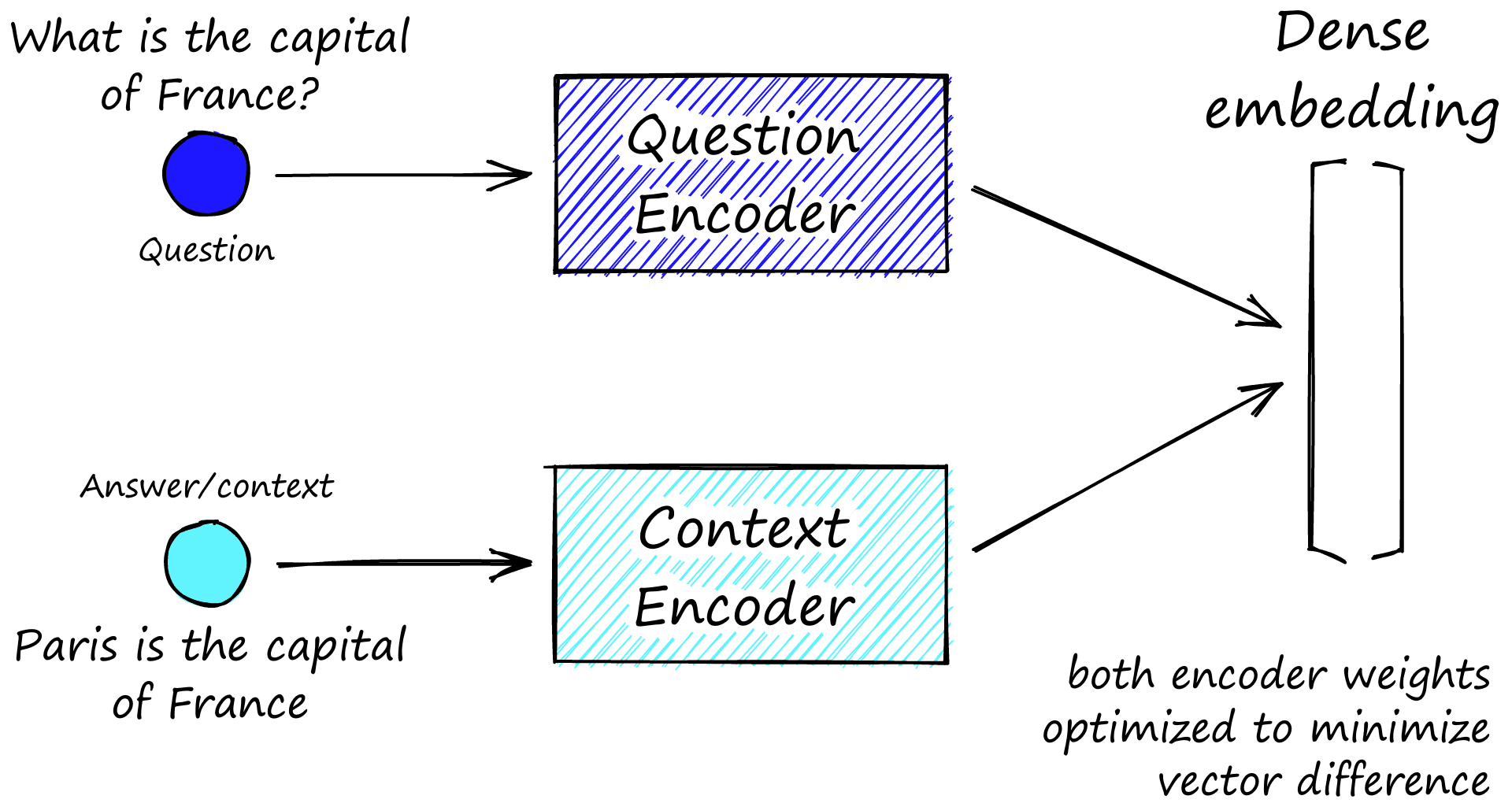
Bi-encoder structure of DPR, we have both a question encoder and a context encoder — both are optimized to output the same (or close) embeddings for each question-context pair.

So when we give our question encoder "What is the capital of France?", we would hope that the output vector would be similar to the vector output by our context encoder for "The capital of France is Paris.".

We can’t rely on all of the question-answer relationships on having been seen during training. So when we input a new question such as "What is the capital of Australia?" our model might output a vector that we could think of as similar to "The capital of Australia is ___". When we compare that to context embeddings in our database, this should be similar to "The capital of Australia is Canberra" (or so we hope).

Fast DPR Setup

Let’s take a quick look at building some context and query embeddings with DPR. We’ll be using the transformers library from Hugging Face.

First, we initialize tokenizers and models for both our context (ctx) model and question model.

In[5]:

from transformers import DPRContextEncoder, DPRContextEncoderTokenizer, \
                         DPRQuestionEncoder, DPRQuestionEncoderTokenizer

In[6]:

ctx_model = DPRContextEncoder.from_pretrained('facebook/dpr-ctx_encoder-single-nq-base')
ctx_tokenizer = DPRContextEncoderTokenizer.from_pretrained('facebook/dpr-ctx_encoder-single-nq-base')

question_model = DPRQuestionEncoder.from_pretrained('facebook/dpr-question_encoder-single-nq-base')
question_tokenizer = DPRQuestionEncoderTokenizer.from_pretrained('facebook/dpr-question_encoder-single-nq-base')

Out[6]:

Downloading: 100%|██████████| 492/492 [00:00<00:00, 142kB/s]
Downloading: 100%|██████████| 438M/438M [00:24<00:00, 17.7MB/s]
Downloading: 100%|██████████| 232k/232k [00:00<00:00, 756kB/s]
...
Downloading: 100%|██████████| 28.0/28.0 [00:00<00:00, 7.14kB/s]

Given a question and several contexts we tokenize and encode like so:

In[7]:

questions = [
    "what is the capital city of australia?",
    "what is the best selling sci-fi book?",
    "how many searches are performed on Google?"
]

contexts = [
    "canberra is the capital city of australia",
    "what is the capital city of australia?",
    "the capital city of france is paris",
    "what is the best selling sci-fi book?",
    "sc-fi is a popular book genre read by millions",
    "the best-selling sci-fi book is dune",
    "how many searches are performed on Google?",
    "Google serves more than 2 trillion queries annually",
    "Google is a popular search engine"
]

In[8]:

xb_tokens = ctx_tokenizer(contexts, max_length=256, padding='max_length',
                          truncation=True, return_tensors='pt')
xb = ctx_model(**xb_tokens)

xq_tokens = question_tokenizer(questions, max_length=256, padding='max_length',
                               truncation=True, return_tensors='pt')
xq = question_model(**xq_tokens)

In[9]:

xb.pooler_output.shape, xq.pooler_output.shape

Out[9]:

(torch.Size([9, 768]), torch.Size([3, 768]))

Note that we have included the questions within our contexts to confirm that the bi-encoder architecture is not just producing a straightforward semantic similarity operation as with sentence-transformers.

Now we can compare our query embeddings `xq` against all of our context embeddings `xb` to see which are the most similar with cosine similarity.

In[10]:

import torch

for i, xq_vec in enumerate(xq.pooler_output):
    probs = cos_sim(xq_vec, xb.pooler_output)
    argmax = torch.argmax(probs)
    print(questions[i])
    print(contexts[argmax])
    print('---')

Out[10]:

what is the capital city of australia?
canberra is the capital city of australia
---
what is the best selling sci-fi book?
the best-selling sci-fi book is dune
---
how many searches are performed on Google?
how many searches are performed on Google?
---

Out of our three questions, we returned two correct answers as the very top answer. It’s clear that DPR is not the perfect model, particularly when considering the simple nature of our questions and small dataset for DPR to retrieve from.

On the positive side however, in ODQA we would return many more contexts and allow a reader model to identify the best answers. Reader models can ‘re-rank’ contexts, so retrieving the top context immediately is not required to return the correct answer. If we were to retrieve the most relevant result 66% of the time, it would likely be a good result.

We can also see that despite hiding exact matches to our questions in the contexts, they interfered with only our last question, being correctly ignored by the first two questions.

Vision Transformers

Computer vision (CV) has become the stage for some exciting advances from transformer models — which have historically been restricted to NLP.

These advances look to make transformers the first widely adopted ML models that excel in both NLP and CV. And in the same way that we’ve been creating dense vectors representing language. We can do the same for images — and even encode images and text into the same vector space.

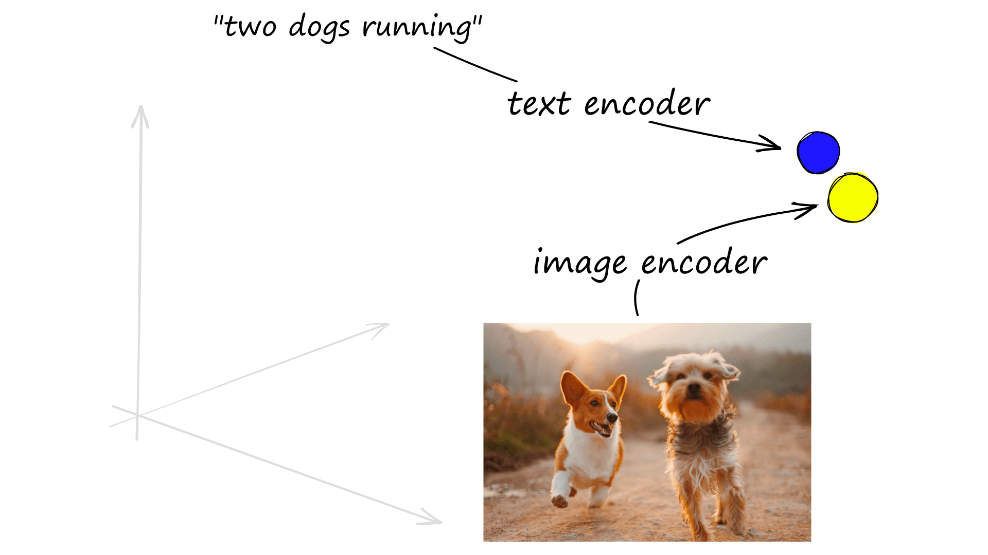
Using specific text and image encoders, we can encode text and images to the same vector space. Photo credit Alvan Nee.

The Vision Transformer (ViT) was the first transformer applied to CV without the assistance of any upstream CNNs (as with VisualBERT [7]). The authors found that ViT can sometimes outperform state-of-the-art (SOTA) CNNs (the long-reigning masters of CV) [8].

These ViT transformers have been used alongside the more traditional language transformers to produce fascinating image and text encoders, as with OpenAI’s CLIP model [9].

The CLIP model uses two encoders like DPR, but this time we use a ViT model as our image encoder and a masked self-attention transformer like BERT for text [10]. As with DPR, these two models are trained in parallel and optimized via a contrastive loss function — producing high similarity vectors for image-text pairs.

That means that we can encode a set of images and then match those images to a caption of our choosing. And we can use the same encoding and cosine similarity logic we have used throughout the article. Let’s go ahead and try.

Image-Text Embedding

Let’s first get a few images to test. We will be using three images of dogs doing different things from Unsplash (links in the caption below).

In[12]:

from PIL import Image
import requests

urls = [
    "https://images.unsplash.com/photo-1576201836106-db1758fd1c97?ixid=MnwxMjA3fDB8MHxwaG90by1wYWdlfHx8fGVufDB8fHx8&ixlib=rb-1.2.1&auto=format&fit=crop&w=400&q=80",
    "https://images.unsplash.com/photo-1591294100785-81d39c061468?ixlib=rb-1.2.1&ixid=MnwxMjA3fDB8MHxwaG90by1wYWdlfHx8fGVufDB8fHx8&auto=format&fit=crop&w=300&q=80",
    "https://images.unsplash.com/photo-1548199973-03cce0bbc87b?ixid=MnwxMjA3fDB8MHxwaG90by1wYWdlfHx8fGVufDB8fHx8&ixlib=rb-1.2.1&auto=format&fit=crop&w=400&q=80"
]

images = [
    Image.open(requests.get(url, stream=True).raw) for url in urls]

# let's see what we have
for image in images:
    plt.show(plt.imshow(np.asarray(image)))

Images downloaded from Unsplash (captions have been manually added — they are not included with the images), photo credits to Cristian Castillo [1, 2] and Alvan Nee.

We can initialize the CLIP model and processor using transformers from Hugging Face.

In[11]:

from transformers import CLIPProcessor, CLIPModel

model = CLIPModel.from_pretrained('openai/clip-vit-base-patch32')
processor = CLIPProcessor.from_pretrained('openai/clip-vit-base-patch32')

Out[11]:

Downloading: 100%|██████████| 3.98k/3.98k [00:00<00:00, 916kB/s]
Downloading: 100%|██████████| 605M/605M [00:44<00:00, 13.6MB/s]
Downloading: 100%|██████████| 316/316 [00:00<00:00, 121kB/s]
...
Downloading: 100%|██████████| 1.49M/1.49M [00:00<00:00, 2.60MB/s]
ftfy or spacy is not installed using BERT BasicTokenizer instead of ftfy.

Now let’s create three true captions (plus some random) to describe our images and preprocess them through our processor before passing them on to our model. We will get output logits and use an argmax function to get our predictions.

In[13]:

captions = ["a dog hiding behind a tree",
            "two dogs running",
            "a dog running",
            "a cucumber on a tree",
            "trees in the park",
            "a cucumber dog"]

inputs = processor(
    text=captions, images=images,
    return_tensors='pt', padding=True
)

outputs = model(**inputs)

probs = outputs.logits_per_image.argmax(dim=1)
probs

In[14]:

for i, image in enumerate(images):
    argmax = probs[i].item()
    print(captions[argmax])
    plt.show(plt.imshow(np.asarray(image)))

Out[14]:

<Figure size 432x288 with 1 Axes>

Out[14]:

a dog hiding behind a tree

Out[14]:

<Figure size 432x288 with 1 Axes>

Out[14]:

<Figure size 432x288 with 1 Axes>

And there, we have flawless image-to-text matching with CLIP! Of course, it is not perfect (our examples here are reasonably straightforward), but it produces some awe-inspiring results in no time at all.

Our model has dealt with comparing text and image embeddings. Still, if we wanted to extract those same embeddings used in the comparison, we access outputs.text_embeds and outputs.image_embeds.

Out[15]:

odict_keys(['loss', 'logits_per_image', 'logits_per_text', 'text_embeds', 'image_embeds', 'text_model_output', 'vision_model_output'])

In[16]:

outputs.text_embeds.shape, outputs.image_embeds.shape

Out[16]:

(torch.Size([6, 512]), torch.Size([3, 512]))

And again, we can follow the same logic as we previously used with cosine similarity to find the closest matches. Let’s compare the embedding for 'a dog hiding behind a tree' with our three images with this alternative approach.

In[17]:

xq = outputs.text_embeds[0]  # 'a dog hiding behind a tree'
xb = outputs.image_embeds

In[18]:

sim = cos_sim(xq, xb)
sim

Out[18]:

tensor([[0.2443, 0.3572, 0.1681]], grad_fn=<MmBackward>)

In[19]:

pred = sim.argmax().item()
pred

In[20]:

plt.show(plt.imshow(np.asarray(images[pred])))

Out[20]:

<Figure size 432x288 with 1 Axes>

As expected, we return the dog hiding behind a tree!

That’s it for this overview of both the early days of dense vector embeddings in NLP and the current SOTA. We’ve covered some of the most exciting applications of both text and image embeddings, such as:

References

[1] T. Mikolov, et al., Efficient Estimation of Word Representations in Vector Space (2013)
[2] T. Mikolov, et al., Linguistic Regularities in Continuous Space Word Representations (2013), NAACL HLT
[3] M. Alcorn, (batter|pitcher)2vec: Statistic-Free Talent Modeling With Neural Player Embeddings (2017), MIT Sloan: Sports Analytics Conference
[4] N. Reimers, I. Girevych, Sentence-BERT: Sentence Embeddings using Siamese BERT-Networks (2019), EMNLP
[5] N. Reimers, SentenceTransformers Documentation, sbert.net
[6] V. Karpukhin, et al., Dense Passage Retrieval for Open-Domain Question Answering (2020), EMNLP
[7] L. H. Li, et al., VisualBERT: A Simple and Performant Baseline for Vision and Language (2019), arXiv
[8] A. Dosovitskiy, et al., An Image is Worth 16x16 Words: Transformers for Image Recognition at Scale (2020), arXiv
[9] A. Radford, et al., CLIP: Connecting Text and Images (2021), OpenAI Blog
[10] CLIP Model Card, Hugging Face
Was this article helpful?