









Have you ever heard of the Gestalt Principles? These are part of a theory of perception that examines how humans group similar objects in order to interpret the complex world around them.
According to the Gestalt principle of proximity, elements that are closer together are perceived to be more related than elements that are farther apart, helping us understand and organize information faster and more efficiently.
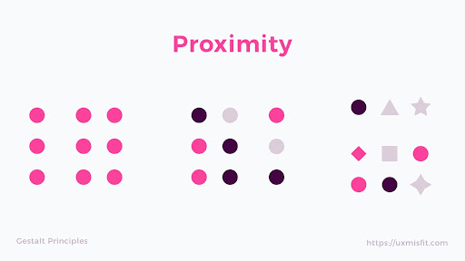
Our brains perceive these sets of closely placed elements as groups. Proximity is essential to our perception.
Likewise, in Machine Learning, the concepts of proximity and similarity are tightly linked. Meaning that the closer two data points are, the more similar they are to one another than to other data points. The content recommendation systems you use every day for movies, texts, songs, and more, rely on this principle.
One Machine Learning algorithm that relies on the concepts of proximity and similarity is K-Nearest Neighbor (KNN). KNN is a supervised learning algorithm capable of performing both classification and regression tasks.
Note: As you’ll see in this article, doing KNN-search or even ANN-search at scale can be slow and expensive. That’s why we made Pinecone — an API for fast, fresh, filtered, and low-cost ANN search at any scale.
As opposed to unsupervised learning — where there is no output variable to guide the learning process and where data is explored by algorithms to find patterns — in supervised learning your existing data is already labeled and you know which behavior you want to predict in the new data you obtain.
The KNN algorithm predicts responses for new data (testing data) based upon its similarity with other known data (training) samples. It assumes that data with similar traits sit together and uses distance measures at its core.
KNN belongs to the class of non-parametric models as it doesn’t learn parameters from the training dataset to come up with a discriminative function to predict new unseen data. It operates by memorizing the training dataset.
Given its flexibility, KNN is used in industries such as:
How near are two data points? It depends on how you measure it, and in Machine Learning, there isn’t just one way of measuring distances.
A distance measure is an objective score that summarizes the relative difference between two objects in a problem domain and plays an important role in most algorithms. Some of the main measures are:
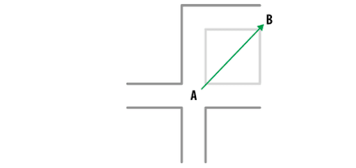
Euclidean distance between two points.
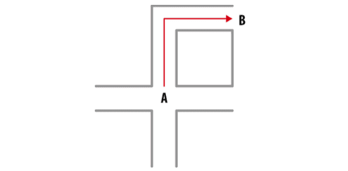
Manhattan distance between two points A and B.
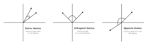
Two cosine vectors that are aligned in the same orientation will have a similarity measurement of 1, whereas two vectors aligned perpendicularly will have a similarity of 0. If two vectors are diametrically opposed, meaning they are oriented in exactly opposite directions (i.e. back-to-back), then the similarity measurement is -1.
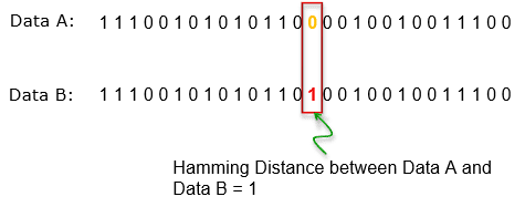
How many bits are different between Data A and Data B? You can easily figure out the difference just by comparing bit by bit. In this case, you would figure out only one bit difference , ande: that’s the Hamming difference between both vectors.
Here is a complete review of different distance measures applied to KNN.
KNN performs classification or regression tasks for new data by calculating the distance between the new example and all the existing examples in the dataset. But how?
Here’s the secret: The algorithm stores the entire dataset and classifies each new data point based on the existing data points that are similar to it. KNN makes predictions based on the training or “known” data only.
After the user defines a distance function, like the ones we mentioned earlier, KNN calculates the distance between data points in order to find the closest data points from our training data for any new data point. The existing data points closest to the new data point using the defined distance will become the “k-neighbors”. For a classification task, KNN will use the most frequent of all values from the k-neighbors to predict the new data label. For a regression task, the algorithm will use the average of all values from the k-neighbors to predict the new data value.
In a classification task with K=3, an unlabelled data point is labeled as pink due to the majority vote of the 3 most similar labeled examples.
All KNN does is store the complete dataset, and without doing any calculation or modeling on top of it, measure the distance between the new data point and its closest data points. For this reason, and since there’s not really a learning process happening, KNN is called a “lazy” algorithm (as opposed to “eager” algorithms like Decision Trees that build generalized models before performing predictions on new data points).
With KNN, in order to make a classification/regression task, you need to define a number of neighbors, and that number is given by the parameter “k”. In other words, “k” determines the number of neighbors the algorithm looks at when assigning a value to any new observation.
This number can go from 1 (in which case the algorithm only looks at the closest neighbor for each prediction) to the total number of data points of the dataset (in which case the algorithm would predict the majority class of the complete dataset).
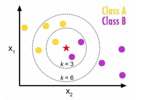
In the above example, if k=3 then the new data point will be classified as B. But if k=6, then it will be classified as A because the majority of points are from class A.
So how can you know the optimum value of “k”? We can decide based on the error calculation of a training and testing set. Separating the data into training and test sets allows for an objective model evaluation.
One popular approach is testing different numbers of “k” and measuring the resulting error, choosing the “k” value at which an increase will cause a very small decrease in the error sum, while a decrease will sharply increase the error sum. This point that defines the optimal number is known as the “elbow point”.
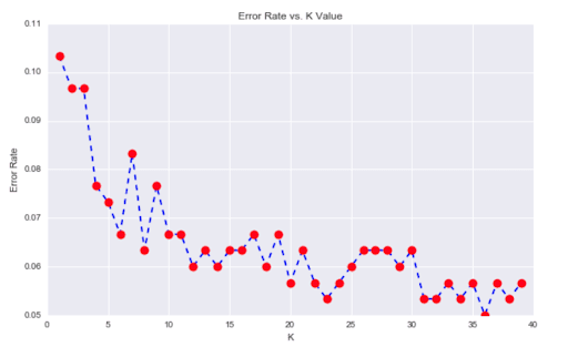
The “k” value best suited for a dataset is selected by using the error rate (this is, the difference between the real and predicted values). After a certain point, the error rate becomes almost constant.
Above, we can see that after “k” > 23, the error rate stabilizes and becomes almost constant. For this reason, “k” = 23 seems to be the optimal value.
Another alternative for deciding the value of “k” is using grid search to find the best value. Grid search is a process that searches exhaustively through a specified numerical space for the algorithm to optimize a given parameter (which in this case is the error rate). Tools like Python’s GridSearchCV can automate the fit of KNN on the training set while validating the performance on the testing set in order to identify the optimal value of “k”.
In contrast to many other Machine Learning algorithms, KNN is simple to implement and intuitive. It’s flexible (has many distance metrics to choose from), evolves as new data is revealed, and has one single hyperparameter to tune (the value of “k”). It can detect linear or nonlinear distributed data, and since it is non-parametric, there are no assumptions to be met to implement it (i.e. as opposed to linear regression models that have plenty of assumptions to be met by the data before they can be employed).
Like every algorithm, it has some downsides. The choice of “k” and the distance metric are critical to its performance and need to be carefully tuned. KNN is also very sensitive to outliers and imbalanced datasets. Also, since all the algorithm does is store the training data to perform its predictions, the memory needs grow linearly with the number of data points you provide for training.
KNN is definitely an algorithm worth learning. Whether it’s for dealing with missing data or predicting image similarity, this is a tool that you can’t miss!
此内容由惯性聚合(RSS阅读器)自动聚合整理,仅供阅读参考。 原文来自 — 版权归原作者所有。