











Locality sensitive hashing (LSH) is a widely popular technique used in approximate similarity search. The solution to efficient similarity search is a profitable one — it is at the core of several billion (and even trillion) dollar companies.
The problem with similarity search is scale. Many companies deal with millions-to-billions of data points every single day. Given a billion data points, is it feasible to compare all of them with every search?
Further, many companies are not performing single searches — Google deals with more than 3.8 million searches every minute[1].
Billions of data points combined with high-frequency searches are problematic — and we haven’t considered the dimensionality nor the similarity function itself. Clearly, an exhaustive search across all data points is unrealistic for larger datasets.
The solution to searching impossibly huge datasets? Approximate search. Rather than exhaustively comparing every pair, we approximate — restricting the search scope only to high probability matches.
Locality Sensitive Hashing
Locality Sensitive Hashing (LSH) is one of the most popular approximate nearest neighbors search (ANNS) methods.
At its core, it is a hashing function that allows us to group similar items into the same hash buckets. So, given an impossibly huge dataset — we run all of our items through the hashing function, sorting items into buckets.
Unlike most hashing functions, which aim to minimize hashing collisions — LSH algorithms aim to maximize hashing collisions.
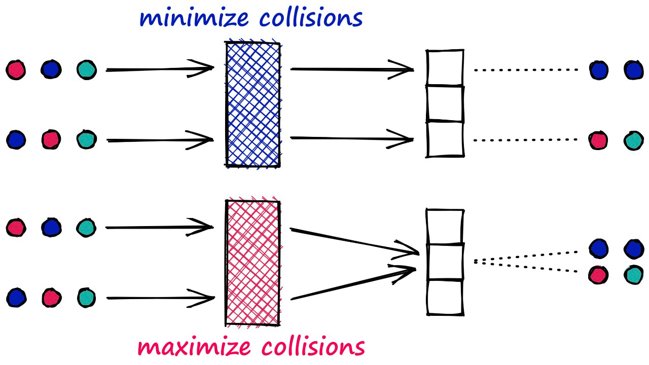
Two hashing functions, the top (blue) minimizes hashing collisions. The bottom (magenta) maximizes hashing collisions — LSH aims to maximize collisions between similar items.
This result for LSH is that similar vectors produce the same hash value and are bucketed together. In contrast, dissimilar vectors will hopefully not produce the same hash value — being placed in different buckets.
Search With LSH
Performing search with LSH consists of three steps:
- Index all of our vectors into their hashed vectors.
- Introduce our query vector (search term). It is hashed using the same LSH function.
- Compare our hashed query vector to all other hash buckets via Hamming distance — identifying the nearest.
At a very high level, that is the process of the LSH methodology we will be covering. However, we will explain all of this in much more detail further in the article.
Effects of Approximation
Before diving into the detail of LSH, we should note that grouping vectors into lower resolution hashed vectors also means that our search is not exhaustive (e.g., comparing every vector), so we expect a lower search quality.
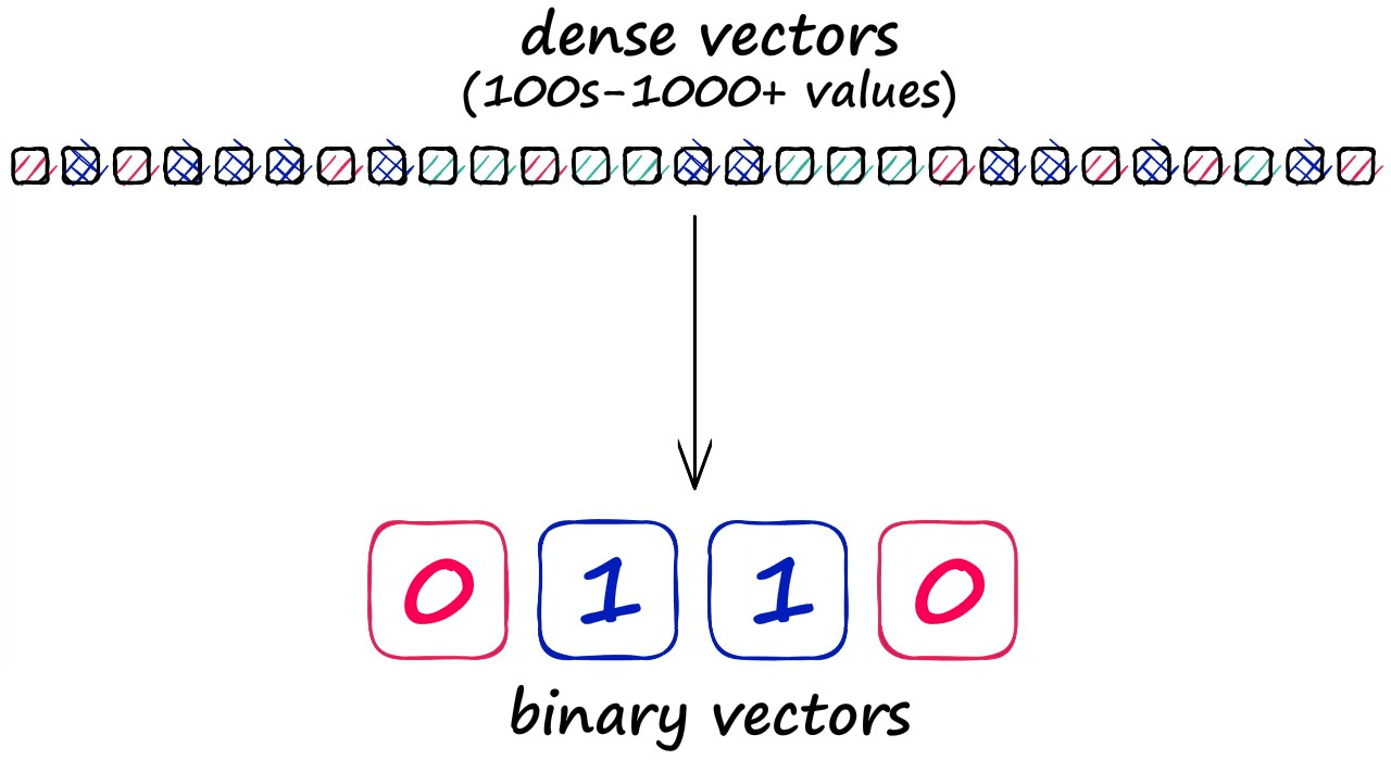
We compress potentially huge dense vectors into highly compressed, grouped binary vectors.
But, the reason for accepting this lower search quality is the potential for significantly faster search speeds.
Which Method?
We’ve been purposely lax on the details here because there are several versions of LSH — each utilizing different hash building and distance/similarity metrics. The two most popular approaches are:
- Shingling, MinHashing, and banded LSH (traditional approach)
- Random hyperplanes with dot-product and Hamming distance
This article will focus on the random hyperplanes method , which is more commonly used and implemented in various popular libraries such as Faiss.
Random Hyperplanes
The random hyperplanes (also called random projection) approach is deceptively simple — although it can be hard to find details on the method.
Let’s learn through an example — we will be using the Sift1M dataset throughout our examples, which you can download using this script.
Now, given a single query vector xq we want to identify the top k nearest neighbors from the xb array.
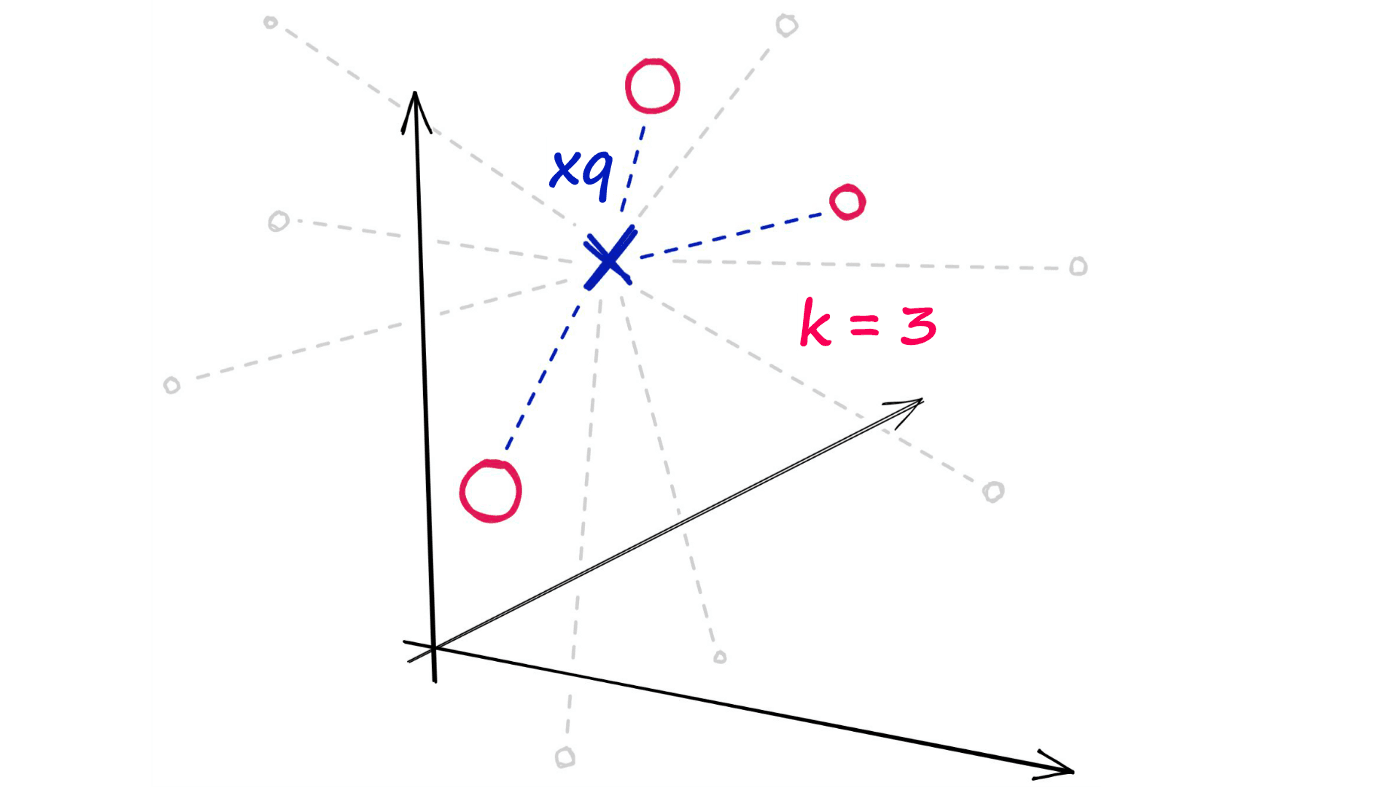
Here we are returning the three nearest neighbors to our query vector xq.
Using the random projection method, we will reduce our highly-dimensional vectors into low-dimensionality binary vectors. Once we have these binary vectors, we can measure the distance between them using Hamming distance.
Let’s work through that in a little more detail.
Creating Hyperplanes
The hyperplanes in this method are used to split our datapoints and assign a value of 0 for those data points that appear on the negative side of our hyperplane — and a value of 1 for those that appear on the positive side.
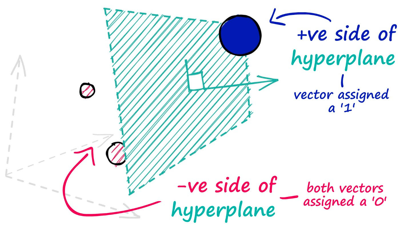
We assign a value of 1 to vectors on the +ve side of our hyperplane and a value of 0 to vectors on the -ve side of the hyperplane.
To identify which side of the hyperplane our data point is located, all we need is the normal vector of the plane — e.g., a vector perpendicular to the plane. We feed this normal vector (alongside our datapoint vector) into a dot product function.
If two vectors share the same direction, the resultant dot product is positive. If they do not share the same direction, it is negative.
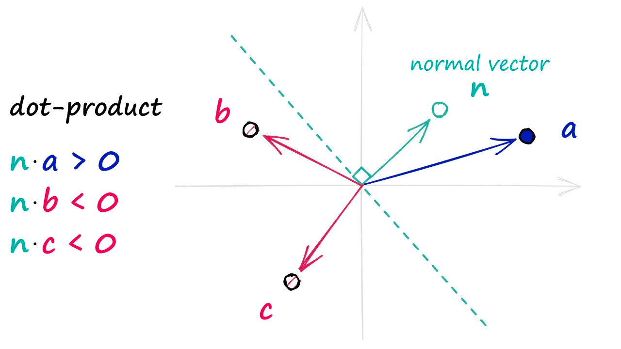
Where our hyperplane normal vector produces a +ve dot-product with another vector, we can view that vector as being in front of the hyperplane. The reverse is true for vectors that produce a -ve dot-product.
In the unlikely case of both vectors being perfectly perpendicular (sitting on the hyperplane edge), the dot product is 0 — we will group this in with our negative direction vectors.
A single binary value doesn’t tell us much about the similarity of our vectors, but when we begin adding more hyperplanes — the amount of encoded information rapidly increases.
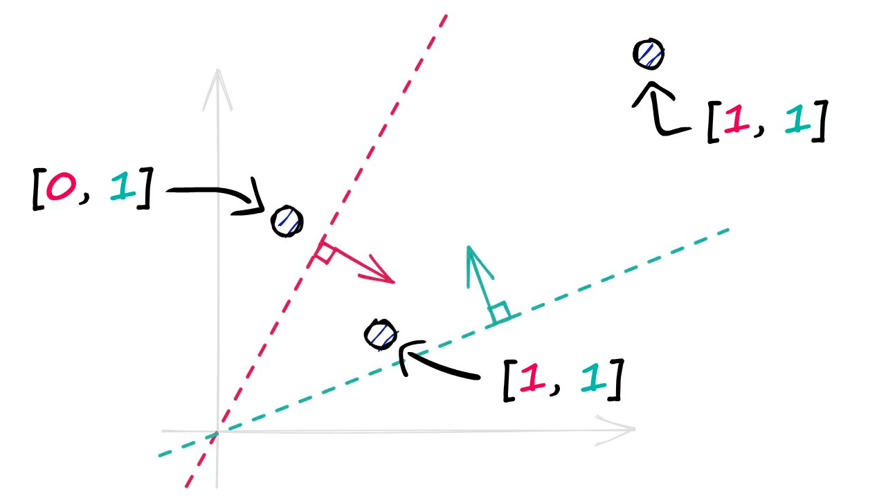
We add more hyperplanes to increase the amount of positional information stored in our binary vectors.
By projecting our vectors into a lower-dimensional space using these hyperplanes, we produce our new hashed vectors.
In the image above, we have used two hyperplanes, and realistically we will need many more — a property that we define using the nbits parameter. We will discuss nbits in more detail later, but for now, we will use four hyperplanes by setting nbits = 4.
Now, let’s create the normal vectors of our hyperplanes in Python.
In[1]:
nbits = 4  # number of hyperplanes and binary vals to produce
d = 2  # vector dimensions
In[2]:
import numpy as np
# create a set of 4 hyperplanes, with 2 dimensions
plane_norms = np.random.rand(nbits, d) - .5
plane_norms
Out[2]:
array([[-0.26623211,  0.34055181],
       [ 0.3388499 , -0.33368453],
       [ 0.34768572, -0.37184437],
       [-0.11170635, -0.0242341 ]])
Through np.random.rand we create a set of random values in the range 0 → 1. We then add -.5 to center our array values around the origin (0, 0). Visualizing these vectors, we see:
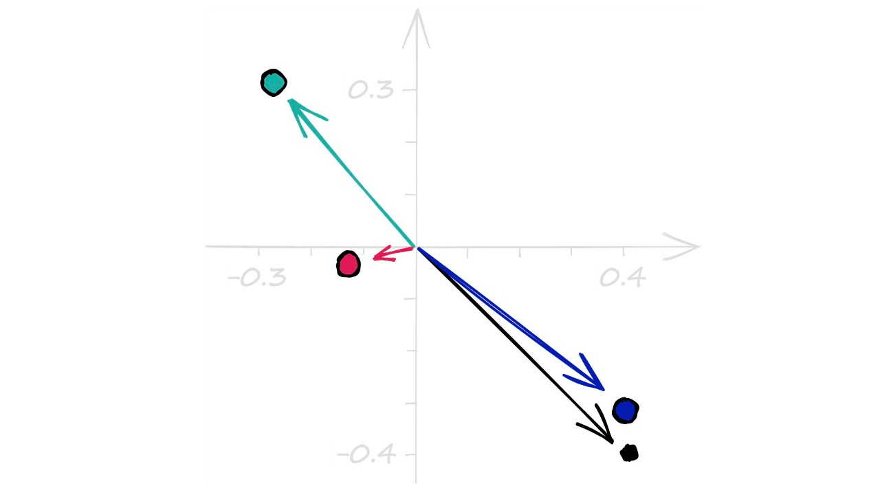
The normal vectors that define the positions of our hyperplanes, which are all centered around the origin (0, 0).
Hashing Vectors
Now let’s add three vectors — a, b, and c — and work through building our hash values using our four normal vectors and their hyperplanes.
In[3]:
a = np.asarray([1, 2])
b = np.asarray([2, 1])
c = np.asarray([3, 1])
In[4]:
# calculate the dot product for each of these
a_dot = np.dot(a, plane_norms.T)
b_dot = np.dot(b, plane_norms.T)
c_dot = np.dot(c, plane_norms.T)
a_dot
Out[4]:
array([ 0.41487151, -0.32851916, -0.39600301, -0.16017455])In[5]:
# we know that a positive dot product == +ve side of hyperplane
# and negative dot product == -ve side of hyperplane
a_dot = a_dot > 0
b_dot = b_dot > 0
c_dot = c_dot > 0
a_dot
Out[5]:
array([ True, False, False, False])In[6]:
# convert our boolean arrays to int arrays to make bucketing
# easier (although is okay to use boolean for Hamming distance)
a_dot = a_dot.astype(int)
b_dot = b_dot.astype(int)
c_dot = c_dot.astype(int)
a_dot
Visualizing this again, we have our three vectors a, b, and c — alongside our four hyperplanes (perpendicular to their respective normal vectors). Taking the +ve and -ve dot-product values for each gives us:
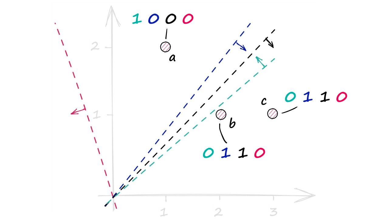
A zero shows that the vector is behind the plane (-ve dot product), and a one shows that the vector is in front of the plane (+ve dot product). We combine these to create our binary vectors.
Which produces our hashed vectors. Now, LSH uses these values to create buckets — which will contain some reference back to our vectors (Eg their IDs). Note that we do not store the original vectors in the buckets — which would significantly increase the size of our LSH index.
As we will see with implementations such as Faiss — the position/order that we added the vector is usually stored. We will use this same approach in our examples.
In[10]:
vectors = [a_dot, b_dot, c_dot]
buckets = {}
i = 0

for i in range(len(vectors)):
    # convert from array to string
    hash_str = ''.join(vectors[i].astype(str))
    # create bucket if it doesn't exist
    if hash_str not in buckets.keys():
        buckets[hash_str] = []
    # add vector position to bucket
    buckets[hash_str].append(i)

print(buckets)
Out[10]:
{'1000': [0], '0110': [1, 2]}
Now that we have bucketed our three vectors, let’s consider the change in the complexity of our search. Let’s say we introduce a query vector that gets hashed as 0111.
With this vector, we compare it to every bucket in our LSH index — which in this case is only two values — 1000 and 0110. We then use Hamming distance to find the closest match, and this happens to be 0110.
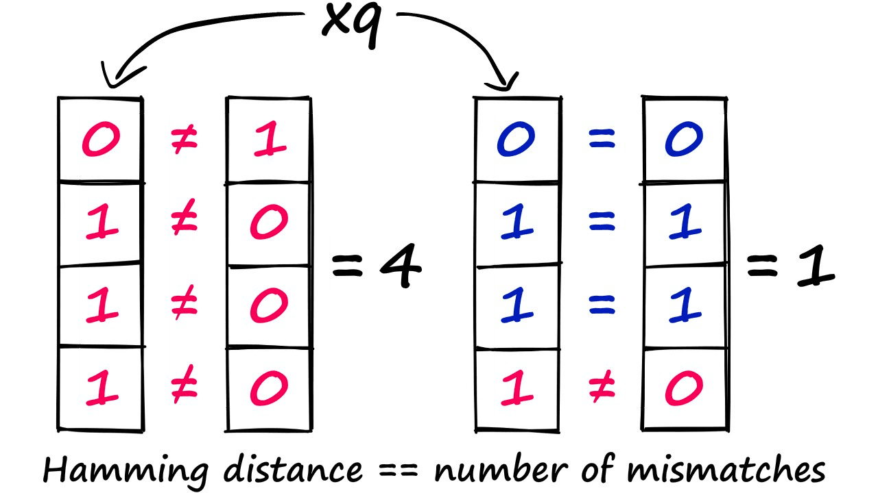
Hamming distance, there are four mismatches between the first two vectors — resulting in a Hamming distance of four. The next two contain just one mismatch, giving a Hamming distance of one.
We have taken a linear complexity function, which required us to compute the distance between our query vector and all of the previously indexed vectors — to a sub-linear complexity — as we no longer need to compute the distance for every vector — because they’re grouped into buckets.
Now, at the same time, vectors 1 and 2 are both equal to 0110. So we cannot possibly find which of those is closest to our query vector. This means there is a degree of search quality being lost — however, this is simply the cost of performing an approximate search. We trade quality for speed.
Balancing Quality vs. Speed
As is often the case in similarity search, a good LSH index requires balancing search quality vs. search speed.
We saw in our mini-example that our vectors were not easy to differentiate, because out of a total of three vectors — random projection had hashed two of them to the same binary vector.
Now imagine we scale this same ratio to a dataset containing one million vectors. We introduce our query vector xq — hash it and calculate the hamming distance between that (0111) and our two buckets (1000 and 0110).
Wow, a million sample dataset searched with just two distance calculations? That’s fast.
Unfortunately, we return around 700K samples, all with the same binary vector value of 0110. Fast yes, accurate — not at all.
Now, in reality, using an nbits value of 4 would produce 16 buckets:
In[1]:
nbits = 4

# this returns number of binary combos for our nbits val
1 << nbits
In[2]:
# we can print every possible bucket given our nbits value like so
for i in range(1 << nbits):
    # get binary representation of integer
    b = bin(i)[2:]
    # pad zeros to start of binary representtion
    b = '0' * (nbits - len(b)) + b
    print(b, end=' | ')
Out[2]:
0000 | 0001 | 0010 | 0011 | 0100 | 0101 | 0110 | 0111 | 1000 | 1001 | 1010 | 1011 | 1100 | 1101 | 1110 | 1111 | We stuck with the two buckets of 1000 and 0110 solely for dramatic effect. But even with 16 buckets — 1M vectors split into just 16 buckets still produces massively imprecise buckets.
In reality, we use many more hyperplanes — more hyperplanes mean higher resolution binary vectors — producing much more precise representations of our vectors.
We control this resolution through hyperplanes with the nbits value. A higher nbits value improves search quality by increasing the resolution of hashed vectors.
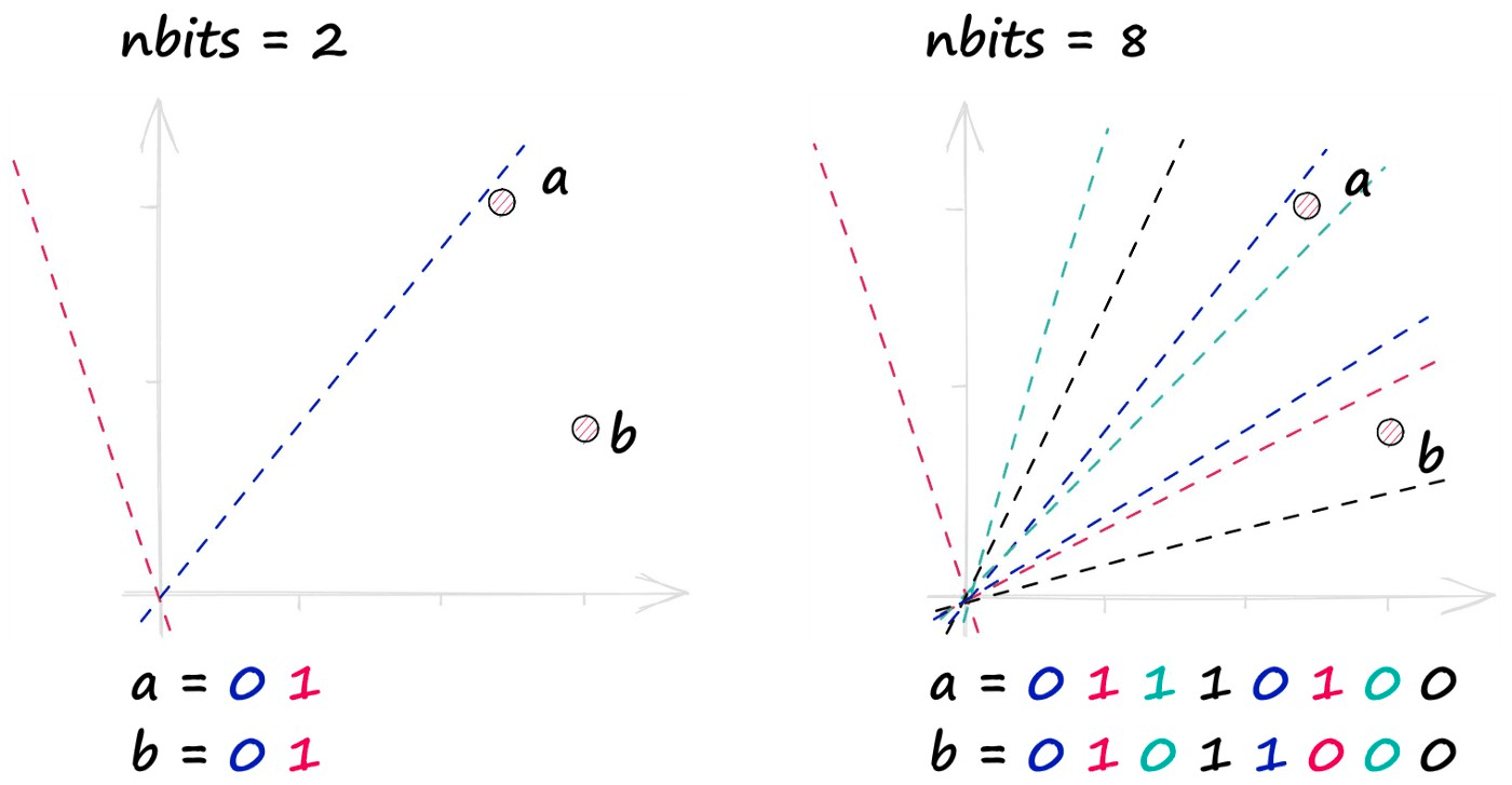
Increasing the nbits parameter increases the number of hyperplanes used to build the binary vector representations.
Adding more possible combinations of hash values increases the potential number of buckets , increasing the number of comparisons and, therefore, search time.
In[1]:
for nbits in [2, 4, 8, 16]:
    print(f"nbits: {nbits}, buckets: {1 << nbits}")
Out[1]:
nbits: 2, buckets: 4
nbits: 4, buckets: 16
nbits: 8, buckets: 256
nbits: 16, buckets: 65536
It’s worth noting that not all buckets will necessarily be used — particularly with higher nbits values. We will see through our Faiss implementation that a nbits value of 128 or more is completely valid and still faster than using a flat index.
There is also this notebook that covers a simple implementation of LSH in Python.
LSH in Faiss
We have discussed Faiss before, but let’s briefly recap. Faiss — or Facebook AI Similarity Search — is an open-source framework built for enabling similarity search.
Faiss has many super-efficient implementations of different indexes that we can use in similarity search. That long list of indexes includes IndexLSH — an easy-to-use implementation of everything we have covered so far.
We initialize our LSH index and add our Sift1M dataset wb like so:
In[3]:
import faiss

d = wb.shape[1]
nbits = 4

# initialize the index using our vectors dimensionality (128) and nbits
index = faiss.IndexLSH(d, nbits)
# then add the data
index.add(wb)
Once our index is ready, we can begin searching using index.search(xq, k) — where xq is our one-or-more query vectors, and k is the number of nearest matches we’d like to return.
In[4]:
xq0 = xq[0].reshape(1, d)
# we use the search method to find the k nearest vectors
D, I = index.search(xq0, k=10)
# the indexes of these vectors are returned to I
I
Out[4]:
array([[26, 47, 43, 2, 6, 70, 73, 74, 25, 0]])The search method returns two arrays. Index positions I (e.g., row numbers from wb) of our k best matches. And the distances D between those best matches and our query vector xq0.
Measuring Performance
Because we have those index positions in I, we can retrieve the original vectors from our array wb.
In[7]:
# we can retrieve the original vectors from wb using I
wb[I[0]]
Out[7]:
array([[31., 15., 47., ...,  0.,  1., 19.],
       [ 0.,  0.,  0., ...,  0., 30., 72.],
       [22., 15., 43., ...,  0.,  0., 12.],
       ...,
       [ 6., 15.,  9., ..., 12., 17., 21.],
       [33., 22.,  8., ...,  0., 11., 69.],
       [ 0., 16., 35., ..., 25., 23.,  1.]], dtype=float32)
In[8]:
# and calculate the cosine similarity between these and xq0
cosine_similarity(wb[I[0]], xq0)
Out[8]:
array([[0.7344476 ],
       [0.6316513 ],
       [0.6995599 ],
       [0.20448919],
       [0.3054034 ],
       [0.25432232],
       [0.30497947],
       [0.341374  ],
       [0.6914262 ],
       [0.26704744]], dtype=float32)
And from those original vectors, we see if our LSH index is returning relevant results. We do this by measuring the cosine similarity between our query vector xq0 and the top k matches.
There are vectors in this index that should return similarity scores of around 0.8. We’re returning vectors with similarity scores of just 0.2 — why do we see such poor performance?
Diagnosing Performance Issues
We know that the nbits value controls the number of potential buckets in our index. When initializing this index, we set nbits == 4 — so all of our vectors must be stored across 4-digit, low-resolution buckets.
If we try to cram 1M vectors into just 16 hash buckets, each of those buckets very likely contain 10–100K+ vectors.
So, when we hash our search query, it matches one of these 16 buckets perfectly — but the index cannot differentiate between the huge number of vectors crammed into that single bucket — they all have the same hashed vector!
We can confirm this by checking our distances D:
Out[10]:
array([[0., 0., 0., 0., 0., 0., 0., 0., 0., 0.]], dtype=float32)We return a perfect distance score of zero for every item — but why? Well, we know that the Hamming distance can only be zero for perfect matches — meaning all of these hashed vectors must be identical.
If all of these vectors return a perfect match, they must all have the same hash value. Therefore, our index cannot differentiate between them — they all share the same position as far as our LSH index is concerned.
Now, if we were to increase k until we return a non-zero distance value, we should be able to infer the number of vectors that have been bucketed with this same hash code. Let’s go ahead and try it.
In[5]:
k = 100
xq0 = xq[0].reshape(1, d)

while True:
    D, I = index.search(xq0, k=k)
    if D.any() != 0:
        print(k)
        break
    k += 100
In[6]:
D # we will see both 0s, and 1sOut[6]:
array([[0., 0., 0., ..., 1., 1., 1.]], dtype=float32)In[7]:
D[:, 172_039:172_041] # we see the hash code switch at position 172_039Out[7]:
array([[0., 1.]], dtype=float32)A single bucket containing 172_039 vectors. That means that we are choosing our top k values at random from those 172K vectors. Clearly, we need to reduce our bucket size.
With 1M samples, which nbits value gives us enough buckets for a more sparse distribution of vectors? It’s not possible to calculate the exact distribution, but we can take an average:
In[11]:
for nbits in [2, 4, 8, 16, 24, 32]:
    buckets = 1 << nbits
    print(f"nbits == {nbits}")
    print(f"{wb.shape[0]} / {buckets} = {wb.shape[0]/buckets}")
Out[11]:
nbits == 2
1000000 / 4 = 250000.0
nbits == 4
1000000 / 16 = 62500.0
nbits == 8
1000000 / 256 = 3906.25
nbits == 16
1000000 / 65536 = 15.2587890625
nbits == 24
1000000 / 16777216 = 0.059604644775390625
nbits == 32
1000000 / 4294967296 = 0.00023283064365386963
With an nbits value of 16 we’re still getting an average of 15.25 vectors within each bucket — which seems better than it is. We must consider that some buckets will be significantly larger than others, as different regions will contain more vectors than others.
Realistically, the nbits values of 24 and 32 may be our tipping point towards genuinely effective bucket sizes. Let’s find the mean cosine similarity for each of these values.
In[11]:
xq0 = xq[0].reshape(1, d)
k = 100

for nbits in [2, 4, 8, 16, 24, 32]:
    index = faiss.IndexLSH(d, nbits)
    index.add(wb)
    D, I = index.search(xq0, k=k)
    cos = cosine_similarity(wb[I[0]], xq0)
    print(np.mean(cos))
Out[11]:
0.5424448
0.560827
0.6372647
0.6676912
0.7162514
0.7048228
It looks like our estimate is correct — the overall similarity for our top 100 vectors experiences a sudden with each nbits increment before leveling off at the nbits == 24 point. But what if we run the process with even larger nbits values?
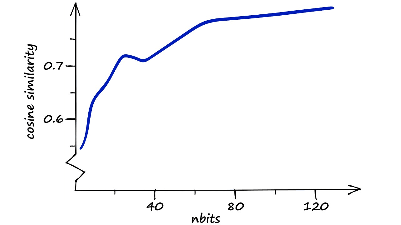
As we increase vector resolution with nbits, our results will become more precise — here, we can see that a larger nbits value results in higher cosine similarity in our results.
Here, the results are apparent. A fast increase in similarity as we declutter the LSH buckets — followed by a slower increase in similarity.
The latter, slower increase in similarity is thanks to the increasing resolution of our hashed vectors. Our buckets are already very sparse — we have many more potential buckets than we have vectors , so we can find little to no performance increase there.
But — we are increasing the resolution and, therefore, the precision of those buckets, so we pull the additional performance from here.
Extracting The Binary Vectors
While investigating our index and the distribution of vectors across our buckets above, we inferred the problem of our bucket sizes. This is useful as we’re using what we have already learned about LSH and can see the effects of the indexes' properties.
However, we can take a more direct approach. Faiss allows us to indirectly view our buckets by extracting the binary vectors representations of wb.
Let’s revert to our nbits value of 4 and see what is stored in our LSH index.
In[2]:
# extract index binary codes (represented as int)
arr = faiss.vector_to_array(index.codes)
arr
Out[2]:
array([ 5, 12, 5, ..., 15, 13, 12], dtype=uint8)In[3]:
# we see that there are 1M of these values, 1 for each vector
arr.shape
In[4]:
# now translate them into the binary vector format
(((arr[:, None] & (1 << np.arange(nbits)))) > 0).astype(int)
Out[4]:
array([[1, 0, 1, 0],
       [0, 0, 1, 1],
       [1, 0, 1, 0],
       ...,
       [1, 1, 1, 1],
       [1, 0, 1, 1],
       [0, 0, 1, 1]])
From this, we can visualize the distribution of vectors across those 16 buckets — showing the most used buckets and a few that are empty.
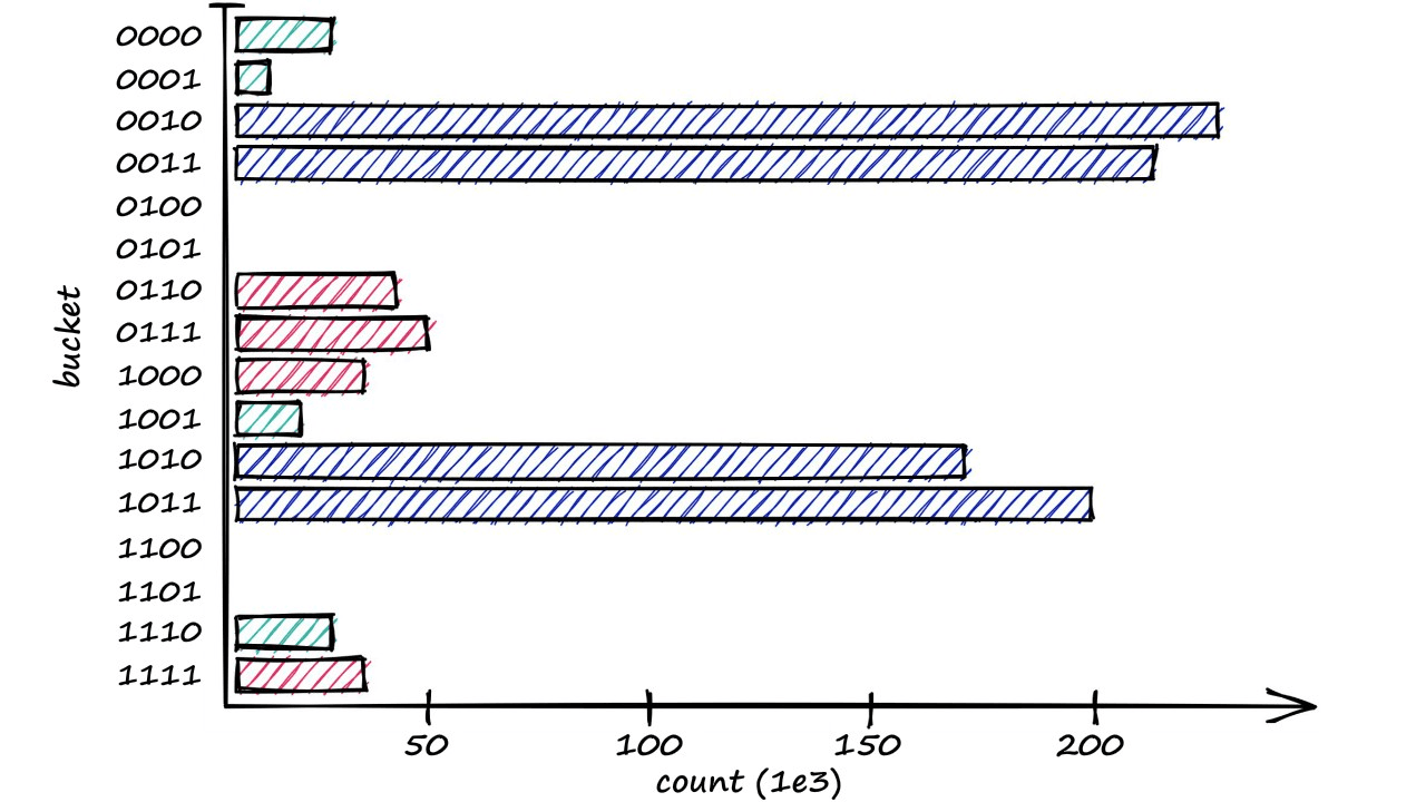
Distribution of vectors in different buckets when nbits == 4.
This and our previous logic are all we need to diagnose the aforementioned bucketing issues.
Where to Use LSH
While LSH can be a swift index, it is less accurate than a Flat index. Using increasingly larger portions of our Sift1M dataset, the best recall score was achieved using an nbits value of 768 (better recall is possible at excessive search times).
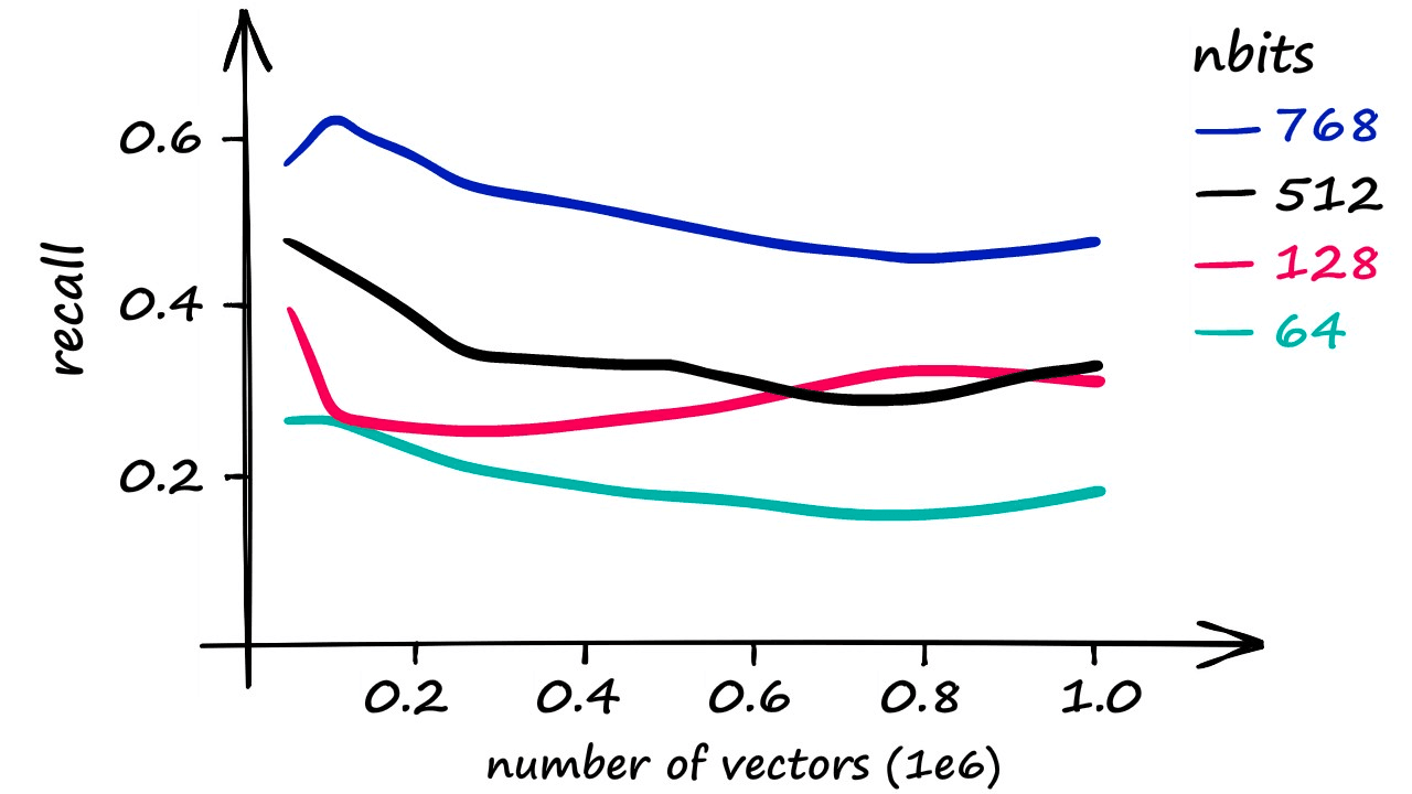
Recall against the number of indexed vectors. The recall is measured as the % of matches with exhaustive search results (using IndexFlatL2).
Although it’s worth noting that using an nbits value of 768 only returns marginally faster results than if using a flat index.
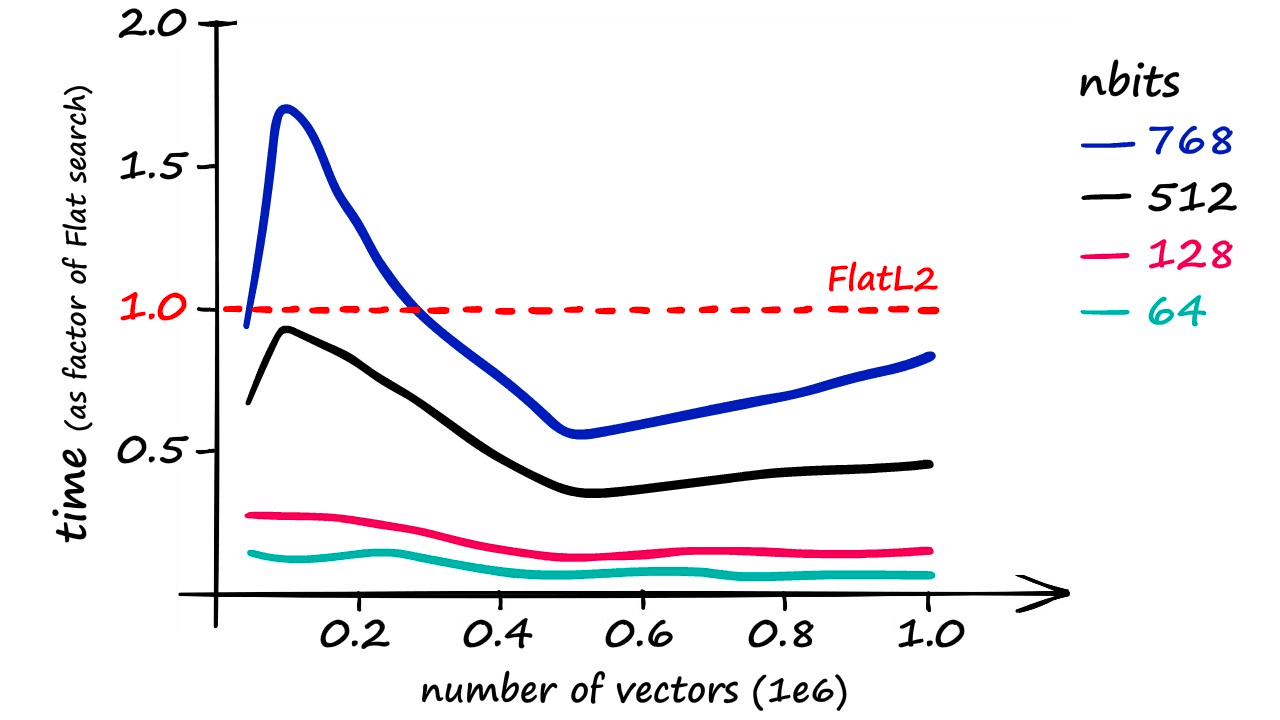
Search time as a factor of search time for IndexFlatL2 at different index sizes and using various nbits values.
More realistic recall rates — while maintaining a reasonable speed increase — are closer to 40%.
However, varying dataset sizes and dimensionality can make a huge difference. An increase in dimensionality means a higher nbits value must be used to maintain accuracy, but this can still enable faster search speeds. It is simply a case of finding the right balance for each use-case and dataset.
Now, of course, there are many options out there for vector similarity search. Flat indexes and LSH are just two of many options — and choosing the right index is a mix of experimentation and know-how.
As always, similarity search is a balancing act between different indexes and parameters to find the best solutions for our use-cases.
We’ve covered a lot on LSH in this article. Hopefully, this has helped clear up any confusion on one of the biggest algorithms in the world of search.
LSH is a complex topic, with many different approaches — and even more implementations available across several libraries.
Beyond LSH, we have many more algorithms suited for efficient similarity search, such as HNSW, IVF, and PQ. You can learn more in our overview of vector search indexes.
References
- Jupyter Notebooks
- [1] Google Searches, Skai.io Blog
Was this article helpful?