





Pinecone lets you add vector search to applications without knowing anything about algorithm optimizations, and it’s free to try. However, we know you like seeing how things work, so enjoy learning about memory-efficient search with product quantization!
Vector similarity search can require huge amounts of memory. Indexes containing 1M dense vectors (a small dataset in today’s world) will often require several GBs of memory to store.
The problem of excessive memory usage is exasperated by high-dimensional data, and with ever-increasing dataset sizes, this can very quickly become unmanageable.
Product quantization (PQ) is a popular method for dramatically compressing high-dimensional vectors to use 97% less memory, and for making nearest-neighbor search speeds 5.5x faster in our tests.
A composite IVF+PQ index speeds up the search by another 16.5x without affecting accuracy, for a whopping total speed increase of 92x compared to non-quantized indexes.
In this article, we will cover all you need to know about PQ: How it works, pros and cons, implementation in Faiss, composite IVFPQ indexes, and how to achieve the speed and memory optimizations mentioned above.
What is Quantization
Quantization is a generic method that refers to the compression of data into a smaller space. I know that might not make much sense — let me explain.
First, let’s talk about dimensionality reduction — which is not the same as quantization.
Let’s say we have a high-dimensional vector, it has a dimensionality of 128. These values are 32-bit floats in the range of 0.0 -> 157.0 (our scope S). Through dimensionality reduction, we aim to produce another, lower-dimensionality vector.
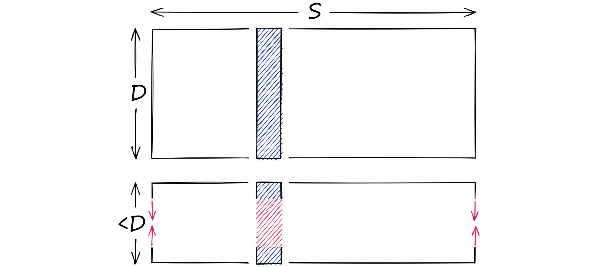
Dimensionality reduction reduces the dimensionality D of vectors, but not the scope S.
On the other hand, we have quantization. Quantization does not care about dimensionality D. Instead, it targets the potential scope of values. Rather than reducing D, we reduce S.
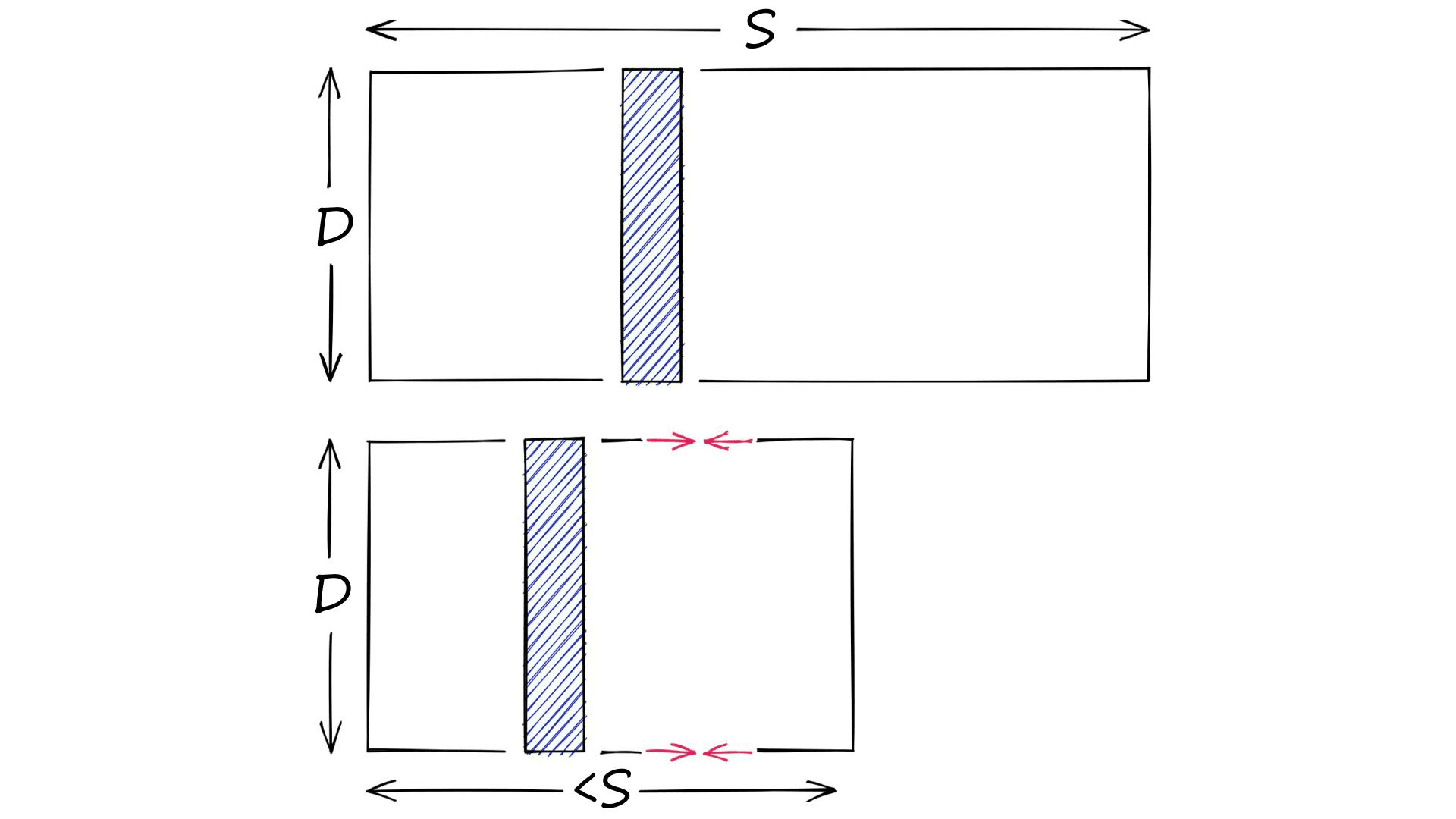
Quantization reduces the scope S of possible vectors. Note that with pre-quantization the scope is typically infinite.
There are many ways of doing this. For example, we have clustering. When we cluster a set of vectors we replace the larger scope of potential values (all possible vectors), with a smaller discrete and symbolic set of centroids.
And this is really how we can define a quantization operation. The transformation of a vector into a space with a finite number of possible values, where those values are symbolic representations of the original vector.
Just to make it very clear, these symbolic representations vary in form. They can be centroids as is the case for PQ, or binary codes like those produced by LSH.
Why Product Quantization?
Quantization is primarily used to reduce the memory footprint of indexes — an important task when comparing large arrays of vectors as they must all be loaded in memory to be compared.
PQ is not the only quantization method that does this, however — but other methods do not manage to reduce memory size as effectively as PQ. We can actually calculate memory usage and quantization operation complexity for PQ and other methods like so:
kmeans = kD PQ = mk^*D^* = k^{1/m}D
We know that D represents the dimensionality of our input vectors, but k and m may be new. k represents the total number of centroids (or codes) that will be used to represent our vectors. And m represents the number of subvectors that we will split our vectors into (more on that later).
(A ‘code’ refers to the quantized representation of our vectors)
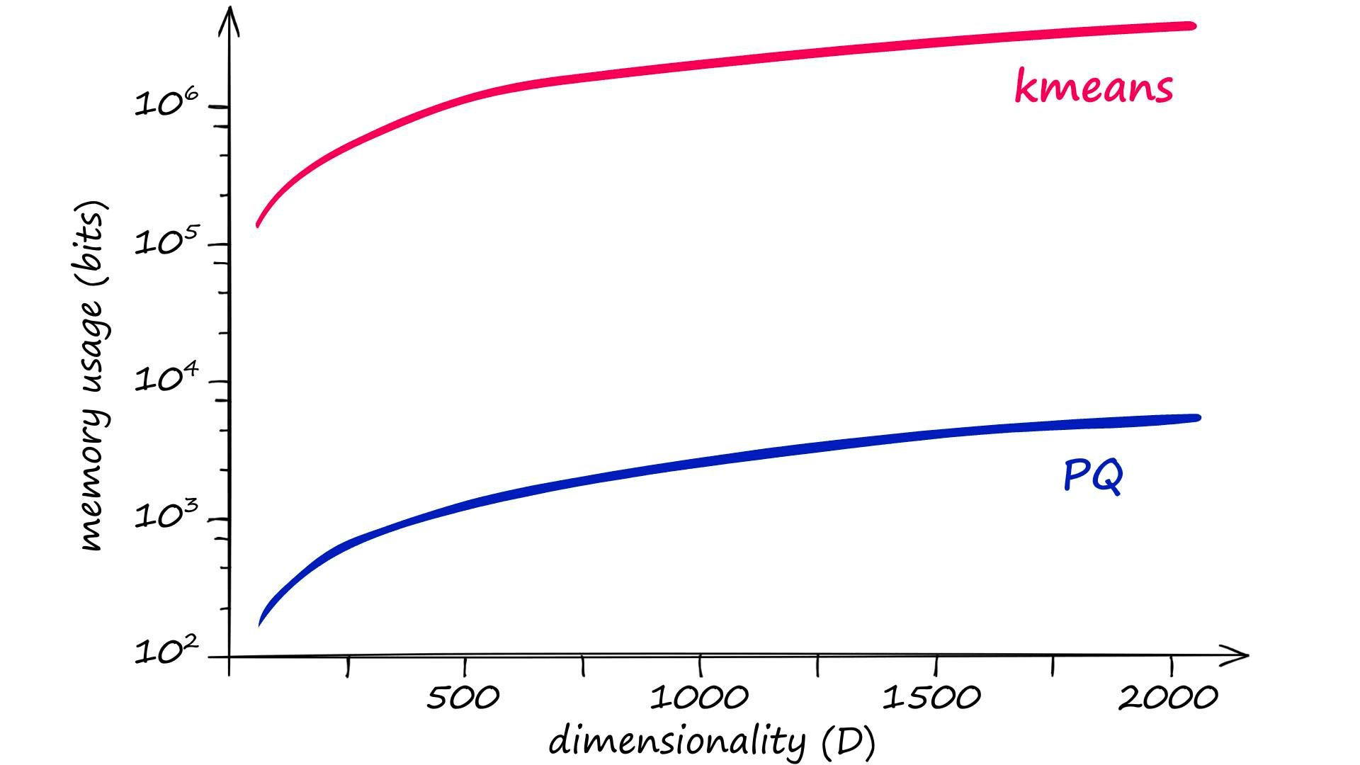
Memory usage (and complexity) vs dimensionality using k=2048 and m=8.
The problem here is that for good results, the recommended k value is of 2048 (211) or more[1]. Given a vector dimensionality of D, clustering without PQ leaves us with very high memory requirements and complexity:
| Operation | Memory and complexity |
|---|---|
| k-means | kD = 2048×128 = 262144 |
| PQ | mkD = (k^(1/m))×D = (2048^(1/8))×128 = 332 |
Given an m value of 8, the equivalent memory usage and assignment complexity for PQ is significantly lower — thanks to the chunking of vectors into subvectors and the subquantization process being applied to those smaller dimensionalities k* and D*, equal to k/m and D/m respectively.
A second important factor is quantizer training. Quantizers require datasets that are several times larger than k for effective training, that is without product subquantization.
Using subquantizers, we only need several multiples of k* (which is k/m) — this can still be a large number — but it can be significantly reduced.
How Product Quantization Works
Let’s work through the logic of PQ. We would usually have many vectors (all of equal length) — but for the sake of simplicity, we will use a single vector in our examples.
In short, PQ is the process of:
- Taking a big, high-dimensional vector,
- Splitting it into equally sized chunks — our subvectors,
- Assigning each of these subvectors to its nearest centroid (also called reproduction/reconstruction values),
- Replacing these centroid values with unique IDs — each ID represents a centroid
High-level view of PQ: Take a big vector, split it into subvectors, assign each to its nearest centroid value, and replace the centroid value with its unique ID — producing a tiny vector of IDs.
At the end of the process, we’ve reduced our highly dimensional vector — that requires a lot of memory — to a tiny vector of IDs that require very little memory.
Our vector is of length D 12. We start by splitting this vector into m subvectors like so:
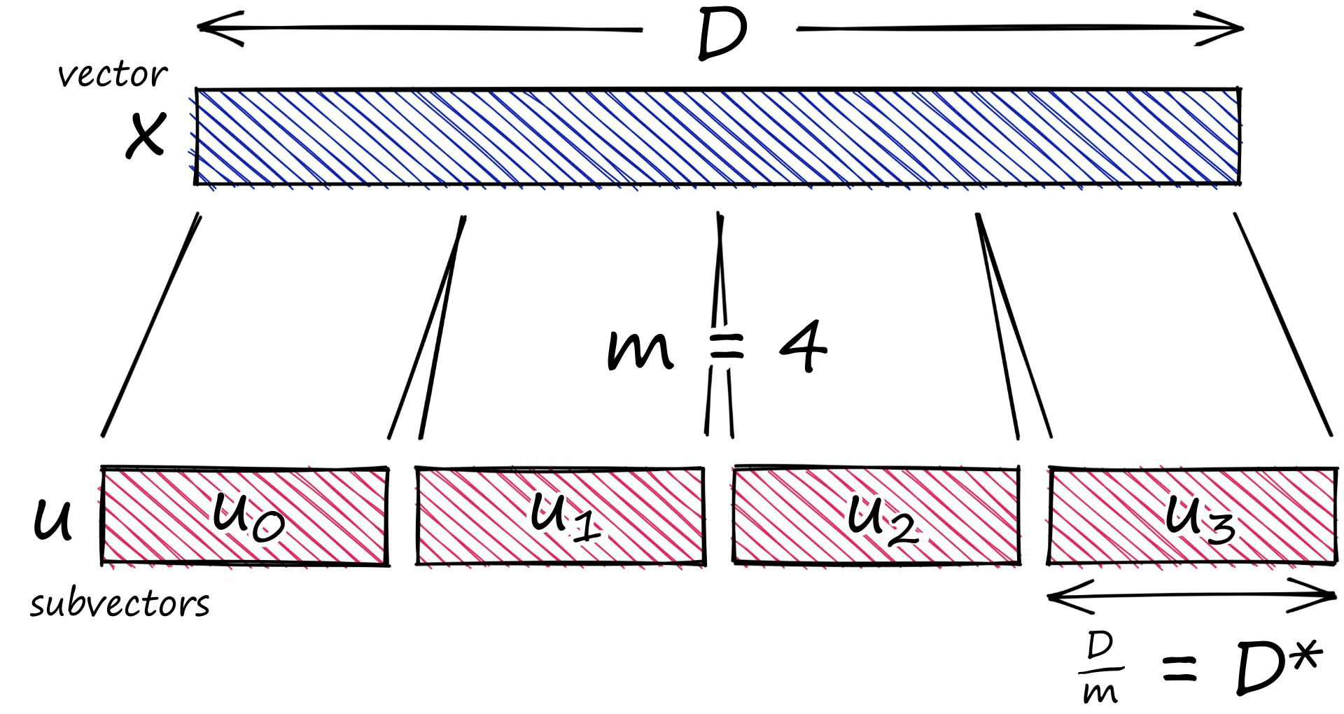
Here we are splitting our high-dimensional vector x into several subvectors u_j.
In[1]:
x = [1, 8, 3, 9, 1, 2, 9, 4, 5, 4, 6, 2]In[2]:
m = 4
D = len(x)
# ensure D is divisable by m
assert D % m == 0
# length of each subvector will be D / m (D* in notation)
D_ = int(D / m)
In[3]:
# now create the subvectors
u = [x[row:row+D_] for row in range(0, D, D_)]
u
Out[3]:
[[1, 8, 3], [9, 1, 2], [9, 4, 5], [4, 6, 2]]We can refer to each subvector by its position j.
For the next part, think about clustering. As a random example, given a large number of vectors we can say “I want three clusters” — and we then optimize these cluster centroids to split our vectors into three categories based on each vector’s nearest centroid.
For PQ we do the same thing with one minor difference. Each subvector space (subspace) is assigned its own set of clusters — and so what we produce is a set of clustering algorithms across multiple subspaces.
In[4]:
k = 2**5
assert k % m == 0
k_ = int(k/m)
print(f"{k=}, {k_=}")
In[5]:
from random import randint

c = []  # our overall list of reproduction values
for j in range(m):
    # each j represents a subvector (and therefore subquantizer) position
    c_j = []
    for i in range(k_):
        # each i represents a cluster/reproduction value position *inside* each subspace j
        c_ji = [randint(0, 9) for _ in range(D_)]
        c_j.append(c_ji)  # add cluster centroid to subspace list
    # add subspace list of centroids to overall list
    c.append(c_j)
Each of our subvectors will be assigned to one of these centroids. In PQ terminology these centroids are called reproduction values and are represented by cⱼ,ᵢ where j is our subvector identifier, and i identifies the chosen centroid (there are k* centroids for each subvector space j).
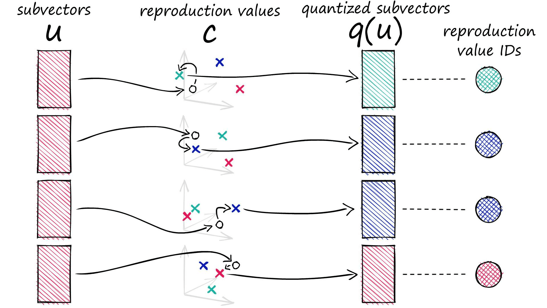
Our subvectors are replaced with a specific centroid vector — which can then be replaced with a unique ID specific to that centroid vector.
In[6]:
def euclidean(v, u):
    distance = sum((x - y) ** 2 for x, y in zip(v, u)) ** .5
    return distance

def nearest(c_j, u_j):
    distance = 9e9
    for i in range(k_):
        new_dist = euclidean(c_j[i], u_j)
        if new_dist < distance:
            nearest_idx = i
            distance = new_dist
    return nearest_idx
In[7]:
ids = []
for j in range(m):
    i = nearest(c[j], u[j])
    ids.append(i)
ids
When we process a vector with PQ, it is split into our subvectors, those subvectors are then processed and assigned to their nearest (sub)cluster centroids (reproduction values).
Rather than storing our quantized vector to be represented by the D*-dimensional centroids, we replace it with a centroid ID. Every centroid cⱼ,ᵢ has its own ID, which can later be used to map those ID values back to the full centroids via our codebook c.
In[8]:
q = []
for j in range(m):
    c_ji = c[j][ids[j]]
    q.extend(c_ji)
Out[9]:
[1, 7, 7, 6, 3, 6, 7, 4, 4, 3, 9, 6]With that, we have compressed a 12-dimensional vector into a 4-dimensional vector of IDs. We have used a small dimensionality here for the sake of simplicity, and so the benefits of such a technique may not be inherently clear.
Let’s switch from our original 12-dimensional vector of 8-bit integers to a more realistic 128-dimensional vector of 32-bit floats (as we will be using throughout the next section). We can find a good balance in performance after compression to an 8-bit integer vector containing just eight dimensions.
Original: 128×32 = 4096 Quantized: 8×8 = 64
That’s a big difference — 64x!
PQ Implementation in Faiss
So far we’ve worked through the logic behind a simple, readable implementation of PQ in Python. Realistically we wouldn’t use this because it is not optimized and we already have excellent implementations elsewhere. Instead, we would use a library like Faiss — or a production-ready service like Pinecone.
We’ll take a look at how we can build a PQ index in Faiss, and we’ll even take a look at combining PQ with an Inverted File (IVF) step to improve search speed.
Before we start, we need to get data. We will be using the Sift1M dataset. It can be downloaded and opened using this script:
In[1]:
import shutil
import urllib.request as request
from contextlib import closing

# first we download the Sift1M dataset
with closing(request.urlopen('ftp://ftp.irisa.fr/local/texmex/corpus/sift.tar.gz')) as r:
    with open('sift.tar.gz', 'wb') as f:
        shutil.copyfileobj(r, f)
In[2]:
import tarfile

# the download leaves us with a tar.gz file, we unzip it
tar = tarfile.open('sift.tar.gz', "r:gz")
tar.extractall()
In[3]:
import numpy as np

# now define a function to read the fvecs file format of Sift1M dataset
def read_fvecs(fp):
    a = np.fromfile(fp, dtype='int32')
    d = a[0]
    return a.reshape(-1, d + 1)[:, 1:].copy().view('float32')
In[4]:
# data we will search through
wb = read_fvecs('./sift/sift_base.fvecs')  # 1M samples
# also get some query vectors to search with
xq = read_fvecs('./sift/sift_query.fvecs')
# take just one query (there are many in sift_learn.fvecs)
xq = xq[0].reshape(1, xq.shape[1])
Now let’s move onto our first index: IndexPQ.
IndexPQ
Our first index is a pure PQ implementation using IndexPQ. To initialize the index we need to define three parameters.
In[2]:
import faiss

D = xb.shape[1]
m = 8
assert D % m == 0
nbits = 8  # number of bits per subquantizer, k* = 2**nbits
index = faiss.IndexPQ(D, m, nbits)
We have our vector dimensionality D, the number of subvectors we’d like to split our full vectors into (we must assert that D is divisible by m).
Finally, we include the nbits parameter. This defines the number of bits that each subquantizer can use, we can translate this into the number of centroids assigned to each subspace as k_ = 2**nbits. An nbits of 11 leaves us with 2048 centroids per subspace.
Because we are using PQ, which uses clustering — we must train our index using our xb dataset.
In[4]:
index.train(xb) # PQ training can take some time when using large nbitsAnd with that, we can go ahead and add our vectors to the index and search.
In[6]:
dist, I = index.search(xq, k)In[7]:
%%timeit
index.search(xq, k)
Out[7]:
1.49 ms ± 49.1 µs per loop (mean ± std. dev. of 7 runs, 1000 loops each)
From our search, we will return the top k closest matches (not the same k used in earlier notation). Returning our distances in dist, and the indices in I.
We can compare the recall performance of our IndexPQ against that of a flat index — which has ‘perfect’ recall (thanks to not compressing vectors and performing an exhaustive search).
In[8]:
l2_index = faiss.IndexFlatL2(D)
l2_index.add(xb)
In[9]:
%%time
l2_dist, l2_I = l2_index.search(xq, k)
Out[9]:
CPU times: user 46.1 ms, sys: 15.1 ms, total: 61.2 ms
Wall time: 15 ms
In[10]:
sum([1 for i in I[0] if i in l2_I])We’re getting 50% which is a reasonable recall if we are happy to sacrifice the perfect results for the reduced memory usage of PQ. There’s also a reduction to just 18% of the flat search time — something that we can improve even further using IVF later.
Lower recall rates are a major drawback of PQ. This can be counteracted somewhat by using larger nbits values at the cost of slower search times and very slow index construction times. However, very high recall is out of reach for both PQ and IVFPQ indexes. If higher recall is required another index should be considered.
How does IndexPQ compare to our flat index in terms of memory usage?
In[11]:
import os

def get_memory(index):
    # write index to file
    faiss.write_index(index, './temp.index')
    # get file size
    file_size = os.path.getsize('./temp.index')
    # delete saved index
    os.remove('./temp.index')
    return file_size
In[12]:
# first we check our Flat index, this should be larger
get_memory(l2_index)
In[13]:
# now our PQ index
get_memory(index)
Memory usage using IndexPQ is — put simply — fantastic, with a memory reduction of 98.4%. It is possible to translate some of these preposterous performance benefits into search speeds too by using an IVF+PQ index.
IndexIVFPQ
To speed up our search time we can add another step, using an IVF index, which will act as the initial broad stroke in reducing the scope of vectors in our search.
After this, we continue our PQ search as we did before — but with a significantly reduced number of vectors. Thanks to minimizing our search scope, we should find we get vastly improved search speeds.
Let’s see how that works. First, we initialize our IVF+PQ index like so:
In[14]:
vecs = faiss.IndexFlatL2(D)

nlist = 2048  # how many Voronoi cells (must be >= k* which is 2**nbits)
nbits = 8  # when using IVF+PQ, higher nbits values are not supported
index = faiss.IndexIVFPQ(vecs, D, nlist, m, nbits)
print(f"{2**nbits=}")  # our value for nlist
We have a new parameter here, nlist defines how many Voronoi cells we use to cluster our already quantized PQ vectors (learn more about IndexIVF here). You may be asking, what on earth is a Voronoi cell — what does any of this even mean? Let’s visualize some 2D ‘PQ vectors’:
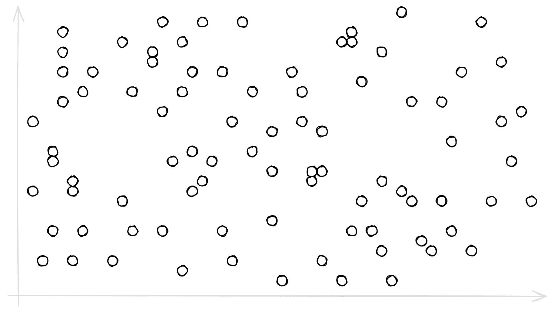
2D chart showing our reconstructed ‘PQ’ vectors. However, in reality, we would never use PQ for 2D vectors as there is simply not enough dimensionality for us to split into subvectors and subquantization.
Let’s add some Voronoi cells:
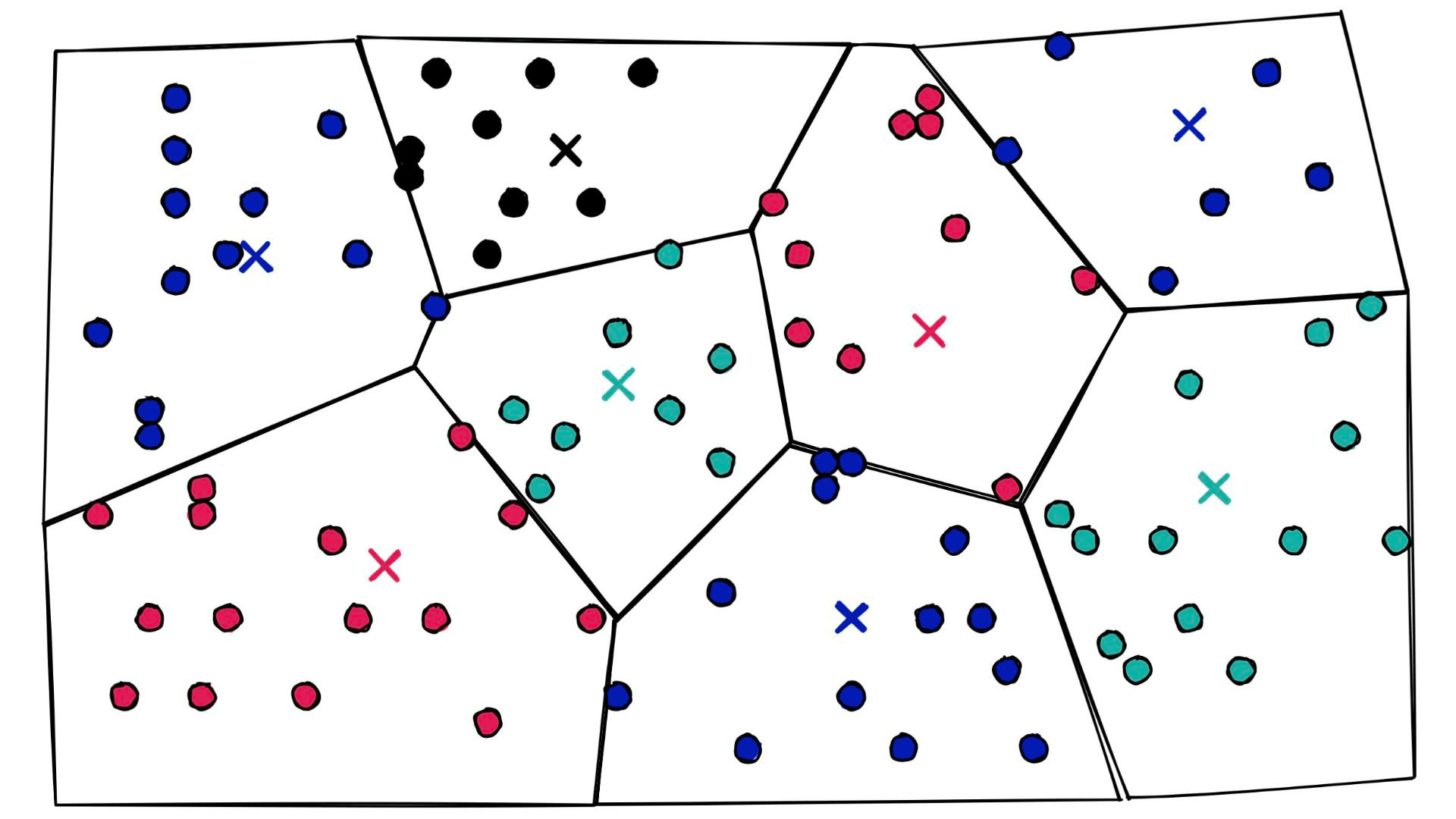
2D chart showing our quantized ‘PQ’ vectors that have now been assigned to different Voronoi cells via IVF.
At a high level, they’re simply a set of partitions. Similar vectors are assigned to different partitions (or cells), and when it comes to search — we introduce our query vector xq and restrict our search to the nearest cell:
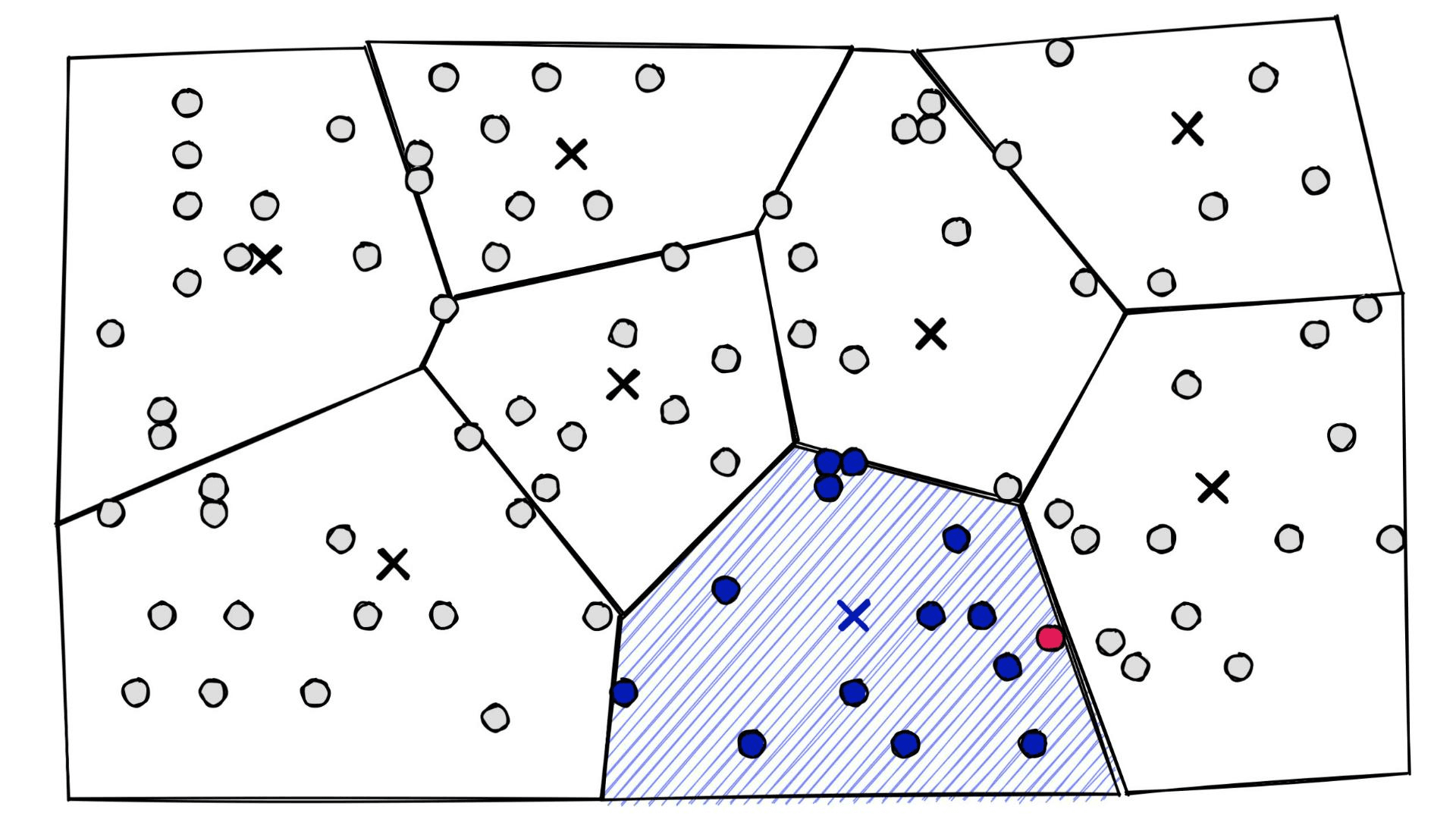
IVF allows us to restrict our search to only vectors that have been assigned nearby cells. The magenta point is our query vector xq. Now let’s go ahead with our train and search — and see how our search speed and recall are doing.
In[18]:
dist, I = index.search(xq, k)In[19]:
%%timeit
index.search(xq, k)
Out[19]:
86.3 µs ± 15 µs per loop (mean ± std. dev. of 7 runs, 10000 loops each)
In[20]:
sum([1 for i in I[0] if i in l2_I])A lightning-fast search time of 86.3μs, but the recall has decreased from our IndexPQ significantly (50% to 34%). Given equivalent parameters, both IndexPQ and IndexIVFPQ should be able to attain equal recall performance.
The secret to improving our recall, in this case, is bumping up the nprobe parameter — which tells us how many of the nearest Voronoi cells to include in our search scope.
2D chart showing our quantized ‘PQ’ vectors that have now been assigned to different Voronoi cells via IVF.
At one extreme, we can include all cells by setting nprobe to our nlist value — this will return the maximum possible recall.
Of course, we don’t want to include all cells. It would make our IVF index pointless as we would then not be restricting our search scope (making this equivalent to a flat index). Instead, we find the lowest nprobe value that achieves this recall performance.
In[22]:
index.nprobe = 2048  # this is searching all Voronoi cells
dist, I = index.search(xq, k)
sum([1 for i in I[0] if i in l2_I])
In[23]:
index.nprobe = 2
dist, I = index.search(xq, k)sum([1 for i in I[0] if i in l2_I])
In[24]:
index.nprobe = 48
dist, I = index.search(xq, k)
sum([1 for i in I[0] if i in l2_I])
With a nprobe of 48, we achieve the best possible recall score of 52% (as demonstrated with nprobe == 2048), while minimizing our search scope (and therefore maximizing search speeds).
By adding our IVF step, we’ve dramatically reduced our search time from 1.49ms for IndexPQ to 0.09ms for IndexIVFPQ. And thanks to our PQ vectors we’ve then paired that with minuscule memory usage that’s 96% lower than the Flat index.
All in all, IndexIVFPQ gave us a huge reduction in memory usage — albeit slightly larger than IndexPQ at 9.2MB vs 6.5MB — and lightning-fast search speeds, all while maintaining a reasonable recall of around 50%.
That’s it for this article! We’ve covered the intuition behind product quantization (PQ), and how it manages to compress our index and enable incredibly efficient memory usage.
We put together the Faiss IndexPQ implementation and tested search times, recall, and memory usage — then optimized the index even further by pairing it with an IVF index using IndexIVFPQ.
| FlatL2 | PQ | IVFPQ | |
|---|---|---|---|
| Recall (%) | 100 | 50 | 52 |
| Speed (ms) | 8.26 | 1.49 | 0.09 |
| Memory (MB) | 256 | 6.5 | 9.2 |
The results of our tests show impressive memory compression and search speeds, with reasonable recall scores.
If you’re interested in learning more about the variety of indexes available in search, including more detail on the IVF index, read our article about the best indexes for similarity search.
References
- [1] H Jégou, et al., Product quantization for nearest neighbor search (2010)
- Jupyter Notebooks
Was this article helpful?