







Language models (LMs) can not rely on language alone. That is the idea behind the “Experience Grounds Language” paper, that proposes a framework to measure LMs' current and future progress. A key idea is that, beyond a certain threshold LMs need other forms of data, such as visual input [1] [2].
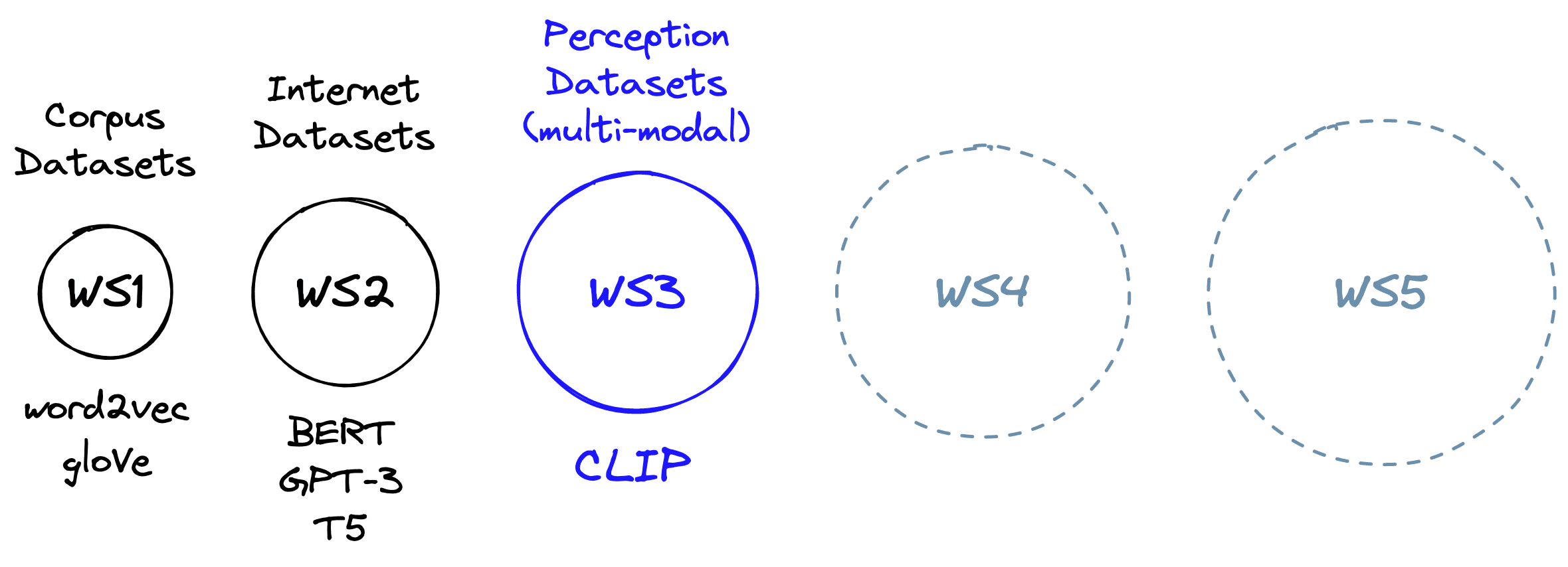
World Scopes (WS), as datasets become larger in scope and span multiple modalities, the capabilities of models trained with them increase.
The next step beyond well-known language models; BERT, GPT-3, and T5 is ”World Scope 3”. In World Scope 3, we move from large text-only datasets to large multi-modal datasets. That is, datasets containing information from multiple forms of media, like both images and text.
The world, both digital and real, is multi-modal. We perceive the world as an orchestra of language, imagery, video, smell, touch, and more. This chaotic ensemble produces an inner state, our “model” of the outside world.
AI must move in the same direction. Even specialist models that focus on language or vision must, at some point, have input from the other modalities. How can a model fully understand the concept of the word “person” without seeing a person?
OpenAI Contrastive Learning In Pretraining (CLIP) is a world scope three model. It can comprehend concepts in both text and image and even connect concepts between the two modalities. In this chapter we will learn about multi-modality, how CLIP works, and how to use CLIP for different use cases like encoding, classification, and object detection.
Multi-modality
The multi-modal nature of CLIP is powered by two encoder models trained to “speak the same language”. Text inputs are passed to a text encoder, and image inputs to an image encoder [3]. These models then create a vector representation of the respective input.
Both models “speak the same language” by encoding similar concepts in text and images into similar vectors. That means that the text “two dogs running across a frosty field” would output a vector similar to an image of two dogs running across a frosty field.
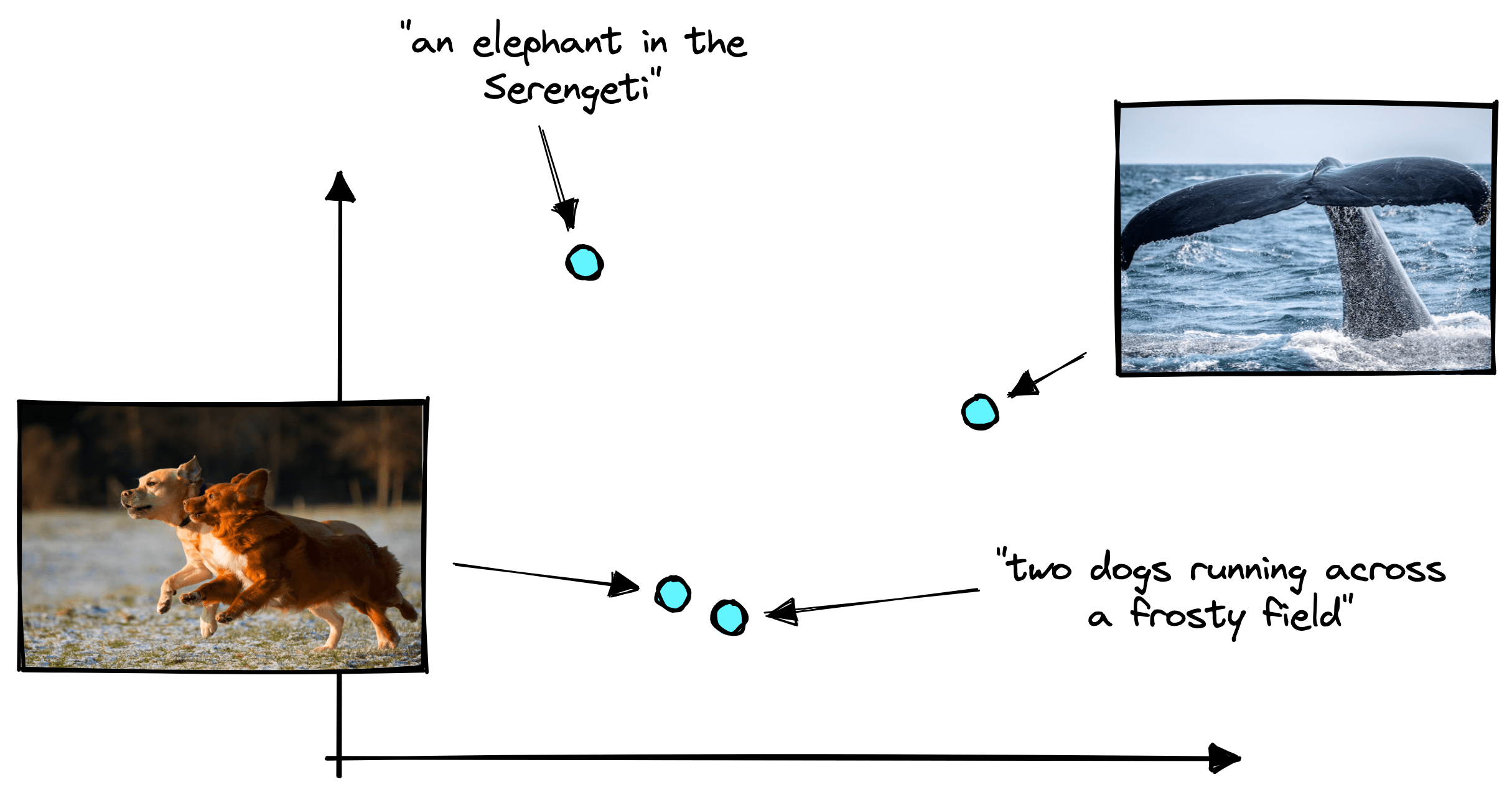
Similar text and images will be encoded into a similar vector space. Dissimilar text and images do not share a similar vector space.
We can think of the language these models speak as the vector space in which they encode vectors. These two models can express nuanced information about text and images through this vector space. However, this “vector language” is far too abstract for us to directly understand.
Rather than directly reading this “language”, we can train other simple neural networks to understand it and make predictions that we can understand. Or we use vector search to identify similar concepts and patterns across text and image domains.
Let’s take a look at an example of CLIP in action.
Text-to-Image Search
Entering a prompt in the search bar above allows us to search through images based on their content rather than any attached textual metadata. We call this Content Based Image Retrieval (CBIR).
With CBIR, we can search for specific phrases such as “two dogs running across a frosty field”. We can even drop the word “dogs” and replace it with everyday slang for dogs like “good boy” or “mans best friend”, and we return the same images showing dogs running across fields.
CLIP can accurately understand language. It understands that in the context of running across a field, we are likely referring to dogs and do not literally mean good children or someone’s “human” best friend.
Amusingly, the dataset contains no images of the food hot dogs (other than one). So, suppose we search for “hot dogs”. In that case, we first get an image containing a hot dog (and a dog), a dog looking toasty in a warm room, another dog looking warm with wooly clothing, and another dog posing for the camera. All of these portray a hot dog in one sense or another.
After being processed by CLIP’s text or image encoder, we are left with vectors. That means we can search across any modality with any modality; we can search in either direction. We can also stick to a single modality, like text-to-text or image-to-image.
Now that we’ve seen what CLIP can do, let’s take a look at how it can do this.
CLIP
CLIP actually consists of two models trained in parallel. A 12-layer text transformer for building text embeddings and a ResNet or vision transformer (ViT) for building image embeddings [3].
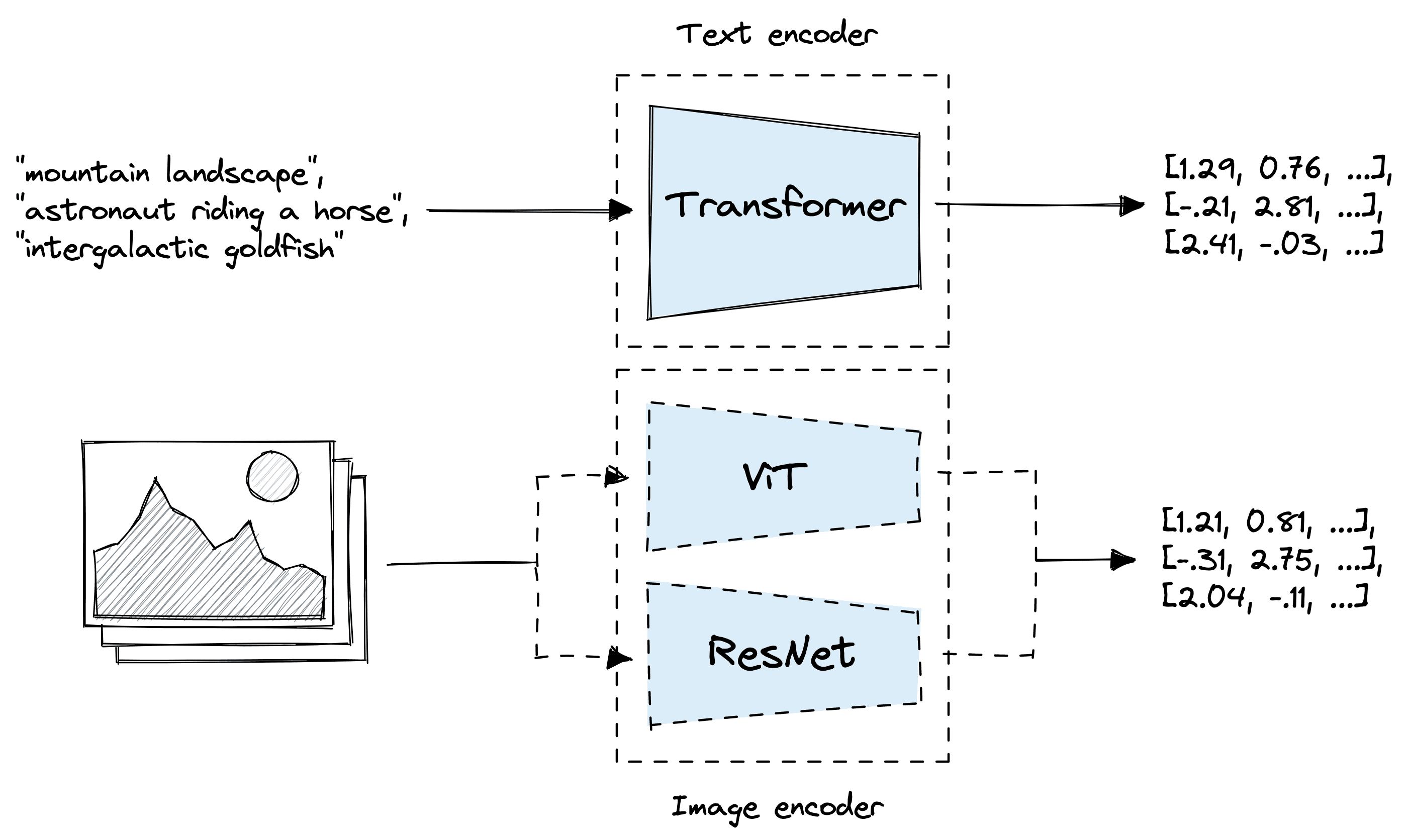
Architecture diagram of CLIP with the text encoder and ViT or ResNet as the image encoder.
The text encoder and image encoder (ResNet or ViT) output single vector embeddings for each text/image record fed into the encoders. All vectors are 512 dimensional and can be represented in the same vector space, meaning similar images and text produce vectors that appear near each other.
Contrastive Pretraining
Across both Natural Language Processing (NLP) and computer vision (CV), large pretrained models dominate the SotA. The idea is that by giving a big model a lot of data, they can learn general patterns from the dataset.
For language models, that may be the general rules and patterns in the English language. For vision models, that may be the characteristics of different scenes or objects.
The problem with multi-modality is that these models are trained separately and, by default, have no understanding of one another. CLIP solves this thanks to image-text contrastive pretraining. With CLIP, text and image encoders are trained while considering the other modality and context. Meaning that the text and image encoders share an “indirect understanding” of patterns in both modalities; language and vision.
Contrastive pretraining works by taking a (text, image) pair – where the text describes the image – and learning to encode the pairs as closely as possible in vector space.
For this to work well, we also need negative pairs to provide a contrastive comparison. We need positive pairs that should output similar vectors and negative pairs that should output dissimilar vectors.
This is the general idea behind contrastive learning, which can be found in the training functions of many models, particularly those that produce embedding vectors.
The negative pairs can be extracted directly from positive pairs. If we have positive pairs and , we simply swap the components, giving us the negative pairs and .
With this, we can apply a loss function that maximizes the similarity between and , and minimizes the similarity between and . Altogether, this looks like this:
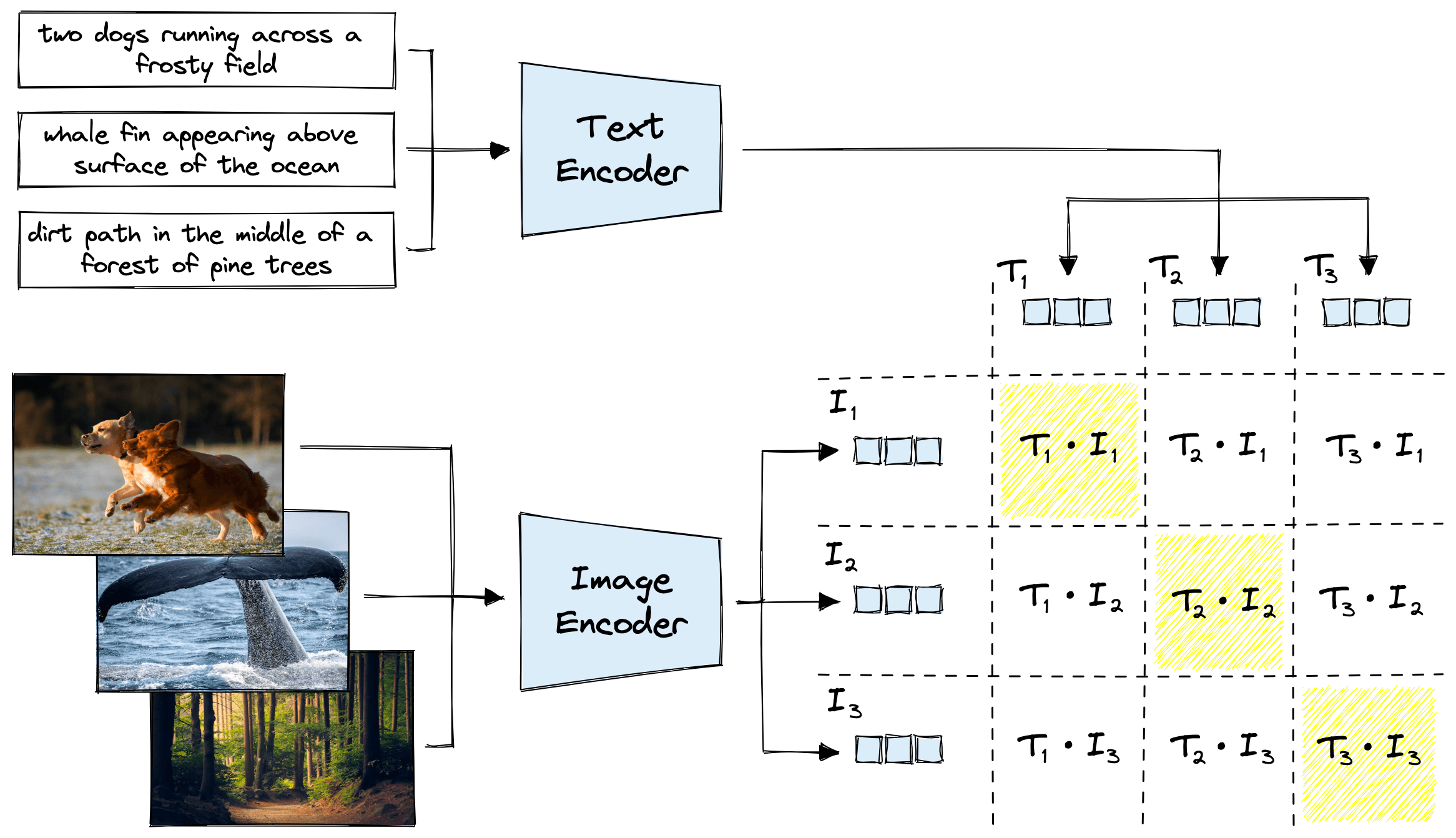
Contrastive pretraining with CLIP.
In this image, we can see a single pretraining step on a single batch. The loss function assumes pairs in the diagonal should have a maximized dot product score, and all other pairs should have a minimized dot product score. Both text and image encoder models are optimized for this.
A fundamental assumption is that there are no other positive pairs within a single batch. For example, we assume that “two dogs running across a frosty field” is only relevant to the image it is paired with. We assume there are no other texts or images with similar meanings.
This assumption is possible because the datasets used for pretraining are diverse and large enough that the likelihood of two similar pairs appearing in a single batch is negligible. Therefore, rare enough to have a little-to-no negative impact on pretraining performance.
Using CLIP
We have a good idea of what CLIP can be used for and how it is trained. With that, how can we get started with it?
OpenAI released a few implementations of CLIP via the Hugging Face library; this is the fastest way to get started. First, we need to install the necessary libraries.
pip install transformers torch datasets
Before we can do anything with CLIP, we need some text and images. The jamescalam/image-text-demo dataset contains a small number of image-text pairs we can use in our examples.
from datasets import load_dataset

data = load_dataset(
    "jamescalam/image-text-demo",
    split="train"
)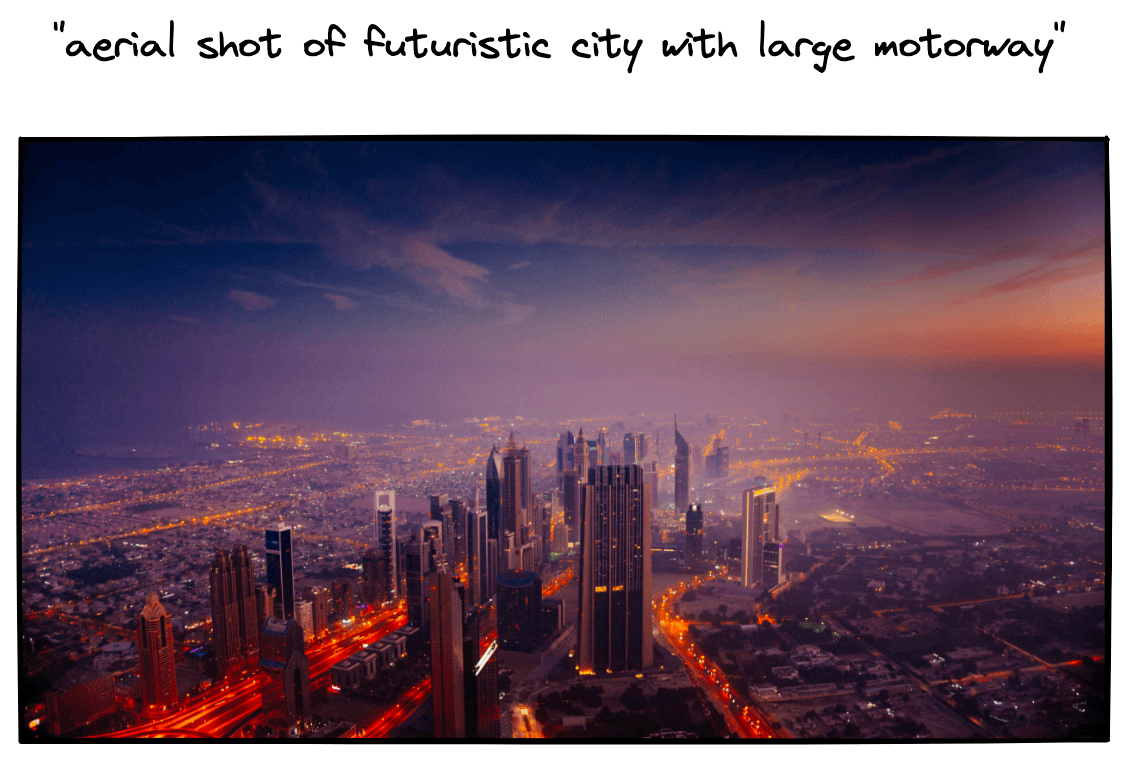
Example of text-image pair found in the dataset. Text is stored in the "text" feature and images in the "image" feature.
With these sample records ready, we can move on to initializing CLIP and an image/text preprocessor like so:
from transformers import CLIPProcessor, CLIPModel
import torch

model_id = "openai/clip-vit-base-patch32"

processor = CLIPProcessor.from_pretrained(model_id)
model = CLIPModel.from_pretrained(model_id)

# move model to device if possible
device = 'cuda' if torch.cuda.is_available() else 'cpu'

model.to(device)
The model is CLIP itself. Note that we use the ViT image encoder (the model is clip-vit). Text and image data cannot be fed directly into CLIP. The text must be preprocessed to create “tokens IDs”, and images must be resized and normalized. The processor handles both of these functions.
Encoding Text
We will start with encoding text using the CLIP text transformer. Before feeding text into CLIP, it must be preprocessed and converted into token IDs. Let’s take a batch of sentences from the unsplash data and encode them.
In[5]:
text = data['text']  # 21

tokens = processor(
    text=text,
    padding=True,
    images=None,
    return_tensors='pt'
).to(device)
tokens.keys()
Out[5]:
dict_keys(['input_ids', 'attention_mask'])This returns the typical text transformer inputs of input_ids and attention_mask.
The input_ids are token ID values where each token ID is an integer value ID that maps to a specific word or sub-word. For example the phrase “multi-modality” may be split into tokens [“multi”, “-”, “modal”, “ity”], which are then mapped to IDs [1021, 110, 2427, 425].
A text transformer maps these token IDs to semantic vector embeddings that the model learned during pretraining.
The attention_mask is a tensor of 1s and 0s used by the model’s internal mechanisms to “pay attention” to real token IDs and ignore padding tokens.
Padding tokens are a special type of token used by text transformers to create input sequences of a fixed length from sentences of varying length. They are appended to the end of shorter sentences, so “hello world” may become “hello world [PAD] [PAD] [PAD]”.
We then use CLIP to encode all of these text descriptions with get_text_features like so:
text_emb = model.get_text_features(
    **tokens
)
One important thing to note here is that these embeddings are not normalized. If we plan on using a similarity metric like the dot product, we must normalize the embeddings:
In[9]:
print(text_emb.shape)
print(text_emb.min(), text_emb.max())
Out[9]:
torch.Size([21, 512])
tensor(-1.1893, grad_fn=<MinBackward1>) tensor(4.8015, grad_fn=<MaxBackward1>)
In[40]:
# IF using dot product similarity, must normalize vectors like so...
import numpy as np

# detach text emb from graph, move to CPU, and convert to numpy array
text_emb = text_emb.detach().cpu().numpy()

# calculate value to normalize each vector by
norm_factor = np.linalg.norm(text_emb, axis=1)
norm_factor.shape
In[41]:
text_emb = text_emb.T / norm_factor
# transpose back to (21, 512)
text_emb = text_emb.T
print(text_emb.shape)
print(text_emb.min(), text_emb.max())
Out[41]:
(21, 512)
-0.1526844 0.53449875
Alternatively, we can use cosine similarity as our metric as this only considers angular similarity and not vector magnitude (like dot product). For our examples, we will normalize and use dot product similarity.
We now have our text embeddings; let’s see how to do the same for images.
Encoding Images
Images will be encoded using the ViT portion of CLIP. Similar to text encoding, we need to preprocess these images using the preprocessor like so:
In[43]:
image_batch = data['image']

images = processor(
    text=None,
    images=image_batch,
    return_tensors='pt'
)['pixel_values'].to(device)
images.shape
Out[43]:
torch.Size([21, 3, 224, 224])Preprocessing images does not produce token IDs like those we saw from preprocessing our text. Instead, preprocessing images consists of resizing the image to a 244x244 array with three color channels (red, green, and blue) and normalizing pixel values into a [0,1][0,1] range.
After preprocessing our images, we get the image features with get_image_features and normalize them as before:
In[44]:
img_emb = model.get_image_features(images)
print(img_emb.shape)
print(img_emb.min(), img_emb.max())
Out[44]:
torch.Size([21, 512])
tensor(-8.6533, grad_fn=<MinBackward1>) tensor(2.6551, grad_fn=<MaxBackward1>)
In[45]:
# NORMALIZE
# detach text emb from graph, move to CPU, and convert to numpy array
img_emb = img_emb.detach().cpu().numpy()

img_emb = img_emb.T / np.linalg.norm(img_emb, axis=1)
# transpose back to (21, 512)
img_emb = img_emb.T
print(img_emb.shape)
print(img_emb.min(), img_emb.max())
Out[45]:
(21, 512)
-0.7275361 0.23383287
With this, we have created CLIP embeddings for both text and images. We can move on to comparing items across the two modalities.
Calculating Similarity
CLIP embedding similarities are represented by their angular similarity. Meaning we can identify similar pairs using cosine similarity:
Or, if we have normalized the embeddings, we can use dot product similarity:
Let’s try both. First, for cosine similarity, we do:
In[46]:
from numpy.linalg import norm

cos_sim = np.dot(text_emb, img_emb.T) / (
    norm(text_emb, axis=1) * norm(img_emb, axis=1)
)
cos_sim.shape
In[47]:
import matplotlib.pyplot as plt

plt.imshow(cos_sim)
plt.show()
Out[47]:
<Figure size 432x288 with 1 Axes>And if we perform the same operation for dot product similarity, we should return the same results:
In[48]:
dot_sim = np.dot(text_emb, img_emb.T)

plt.imshow(cos_sim)
plt.show()
Out[48]:
<Figure size 432x288 with 1 Axes>Both of these similarity score arrays look the same, and if we check for the difference between the two arrays, we will see that the scores are the same. We see some slight differences due to floating point errors.
In[51]:
diff = cos_sim - dot_sim
diff.min(), diff.max()
Using the embedding functions of CLIP in this way, we can perform a semantic search across the modalities of text and image in any direction. We can search for images with text, text with images, text with text, and images with images.
These use cases are great, but we can make slight modifications to this for many other tasks.
Classification
One of the most impressive demonstrations of CLIP is its unparalleled zero-shot performance on various tasks. For example, given the fragment/imagenette dataset from Hugging Face Datasets, we can write a list of brief sentences that align with the ten class labels.
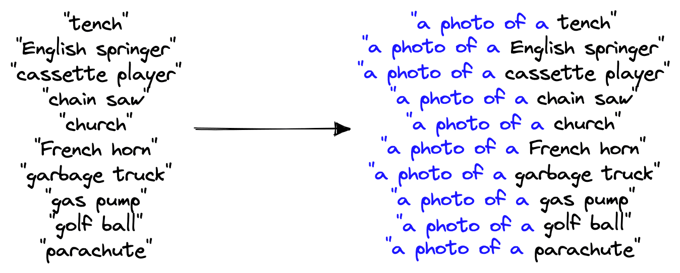
We take the original imagenette labels and preappend "a photo of a ..." to each to create a set of CLIP-friendly sentence representations.
From this, we can calculate the cosine similarity between the text embeddings of these ten labels against an image we’d like to classify. The text that returns the highest similarity is our predicted class.
Object Detection
Another compelling use case of zero-shot CLIP is object detection. We can do this by splitting our images into smaller patches and running each patch through the image encoder of CLIP. We then compare these patch embeddings to a text encoding describing what we are looking for. After calculating the similarity scores for all patches, we can collate them into a map of relevance.
For example, given an image of a butterfly and a cat, we could break it into many small patches. Given the prompt "a fluffy cat", we will return an outline of the cat, whereas the prompt "a butterfly" will produce an outline of the butterfly.
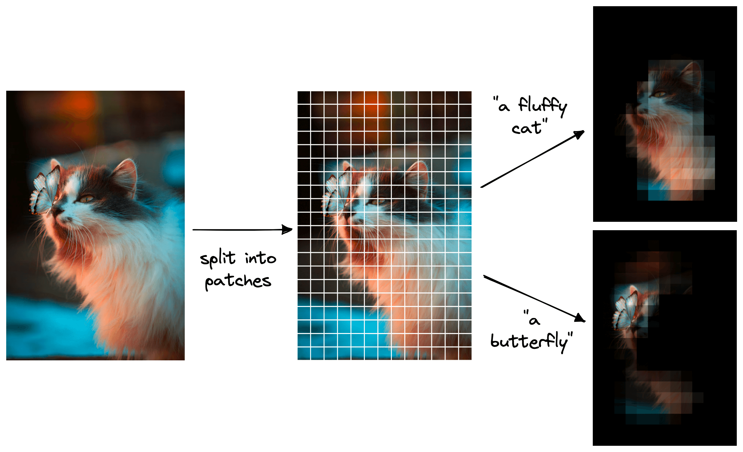
Zero-shot object detection with CLIP allows us to find specific objects with natural language prompts.
These are only a few of the use cases of CLIP and only scratch the surface of what is possible with this model and others in the scope of multi-modal ML.
That’s it for this introduction to multi-modal ML with OpenAI’s CLIP. The past years since the CLIP release have seen ever more fascinating applications of the model.
DALL-E 2 is a well-known example of CLIP. The incredible images generated by DALL-E 2 start by embedding the user’s text prompt with CLIP [4]. That text embedding is then passed to the diffusion model, which generates some mind-blowing images.
The fields of NLP and CV have mainly progressed independently of each other for the past decade. However, with the introduction of world scope three models, they’re becoming more entwined into a majestic multi-modal field of Machine Learning.
Resources
[1] Y. Bisk et al., Experience Grounds Language (2020), EMNLP
[2] J. Alammar, Experience Grounds Language: Improving language models beyond the world of text (2022), YouTube
[3] A. Radford et al., Learning Transferable Visual Models From Natural Language Supervision (2021), arXiv
[4] A. Ramesh, P. Dhariwal, A. Nichol, C. Chu, M. Chen, Hierarchical Text-Conditional Image Generation with CLIP Latents (2022), arXiv
Was this article helpful?