







In the world of vector search, there are many indexing methods and vector processing techniques that allow us to prioritize between recall, latency, and memory usage.
Using specific methods such as IVF, PQ, or HNSW, we can often return good results. But for best performance we will usually want to use composite indexes.
Note: Pinecone lets you build scalable, high-performance vector search into your applications without knowing anything about composite indexes. However, we know you like seeing how things work, so enjoy learning about composite indexes and the Faiss Index Factory!
We can view a composite index as a step-by-step process of vector transformations and one or more indexing methods. Allowing us to place multiple indexes and/or processing steps together to create our ‘ideal’ index.
For example, we can use an inverted file (IVF) index to reduce the scope of our search (increasing search speed), and then add a compression technique such as product quantization (PQ) to keep larger indexes within a reasonable size limit.
Where there is the ability to customize indexes, there is the risk of producing indexes with unnecessarily poor recall, latency, or memory usage.
We must know how composite indexes work if we want to build robust and high-performance vector similarity search applications. It is essential to understand where different indexes or vector transformations can be used — and when they are not needed.
In this article, we will learn how to build high-performance composite indexes using Facebook AI Similarity Search (Faiss) — a powerful library used by many for building fast and accurate vector similarity search indexes. We will also introduce the Faiss index_factory which allows us to build composite indexes with clearer, more elegant code.
What are Composite Indexes
Composite indexes are akin to lego blocks; we place one on top of another. We will find that most blocks fit together — but different combinations can produce anything from an artistic masterpiece to an unrecognizable mess.
The same applies to Faiss. Most components can be placed together — but that does not mean they should be placed together.
A composite index is built from any combination of:
- Vector transform — a pre-processing step applied to vectors before indexing (PCA, OPQ).
- Coarse quantizer — rough organization of vectors to sub-domains (for restricting search scope, includes IVF, IMI, and HNSW).
- Fine quantizer — a finer compression of vectors into smaller domains (for compressing index size, such as PQ).
- Refinement — a final step at search-time which re-orders results using distance calculations on the original flat vectors. Alternatively, another index (non-flat) index can be used.
Note that coarse quantization refers to the ‘clustering’ of vectors (such as inverted indexing with IVF). By using coarse quantization, we enable non-exhaustive search by limiting the search scope.
Fine quantization describes the compression of vectors into codes (as with PQ) [1][2][3]. The purpose of this is to reduce the memory usage of the index.
Index Components
We can build a composite index using the following components:
| Vector transform | Coarse quantizer | Fine quantizer | Refinement |
|---|---|---|---|
| PCA, OPQ, RR, L2norm, ITQ, Pad | IVF,Flat, IMI, IVF,HNSW, IVF,PQ, IVF,RCQ, HNSW,Flat, HNSW,SQ, HNSW,PQ | Flat, PQ, SQ, Residual, RQ, LSQ, ZnLattice, LSH | RFlat, Refine* |
For example, we could build an index where we:
- Transform incoming vectors using
OPQ. - Perform coarse quantization of vectors by storing them in an inverted file list
IVF, enabling non-exhaustive search. - Compress vectors, reducing memory usage with
PQwithin each IVF cell (the vectors are quantized, but their cell assignment does not change). - After the search, re-order results based on their original flat vectors
RFlat.
When building these indexes, it can get messy to use a list of the different Faiss classes — so it is often clearer to build our indexes using the Faiss index_factory.
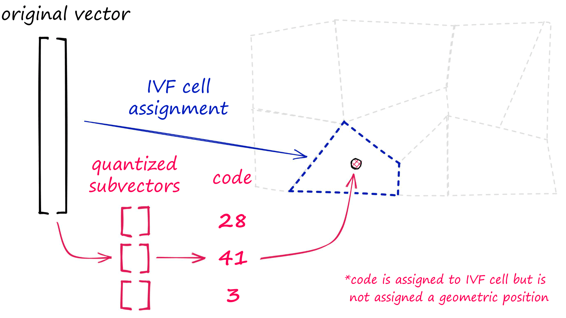
We can merge IVF and PQ indexes to store quantized PQ vectors in an IVF structure.
Faiss Index Factory
The Faiss index_factory function allows us to build composite indexes using little more than a string. It allows us to switch:
quantizer = faiss.IndexFlatL2(128)
index = faiss.IndexIVFFlat(quantizer, 128, 256)
For this:
index_f = faiss.index_factory(128, "IVF256,Flat")We haven’t specified the L2 distance in our index_factory example because the index_factory uses L2 by default. If we’d like to use IndexFlatIP we add faiss.METRIC_INNER_PRODUCT to our index_factory parameters.
We can confirm that both methods produce the same composite index by comparing their performance. First, do they return the same nearest neighbors?
In[4]:
k = 100
D, I = index.search(xq, k)  # search class-based index
In[5]:
D_f, I_f = index_f.search(xq, k) # search index_factory indexIn[6]:
I_f.tolist() == I.tolist() # check that both output same resultsIdentical results, and how do they compare for search speed and memory usage?
In[7]:
%%timeit
index.search(xq, k)
Out[7]:
153 µs ± 7.47 µs per loop (mean ± std. dev. of 7 runs, 10000 loops each)
In[8]:
%%timeit
index_f.search(xq, k)
Out[8]:
148 µs ± 5.79 µs per loop (mean ± std. dev. of 7 runs, 10000 loops each)
The get_memory function returns an exact match for memory usage. Search speeds are incredibly close, with the index_factory version 5µs faster — a negligible difference.
We calculate recall as the percentage of matches from the top-k between a flat L2 index and the tested index.
The more commonly used metric in literature is recall@k; this is not the recall calculated here. Recall@k is the percentage of queries that returned its nearest neighbor in the top k returned records.
If we returned the ground-truth nearest neighbor 50% of the time when using a k value of 100, we would say the recall@100 performance is 0.5.
Why Use the Index Factory
Judging from our tests, we can be confident that these two index-building methods are nothing more than separate paths to the same destination.
With that in mind — why should we care to learn how we use index_factory? First, it can depend on personal preference. If you prefer the class-based index building approach, stick with it.
However, through using the index_factory we can greatly improve the elegance and clarity of our code. We will see that five lines of complicated code can be represented in a single — more readable — line of code when using the index_factory.
Let’s put together a composite index where we pre-process vectors with OPQ, cluster with IVF, quantize using PQ, then re-order with a flat index.
d = xb.shape[1]
m = 32
nbits = 8
nlist = 256

# we initialize our OPQ and coarse+fine quantizer steps separately
opq = faiss.OPQMatrix(d, m)
# d now refers to shape of rotated vectors from OPQ (which are equal)
vecs = faiss.IndexFlatL2(d)
sub_index = faiss.IndexIVFPQ(vecs, d, nlist, m, nbits)
# now we merge the preprocessing, coarse, and fine quantization steps
index = faiss.IndexPreTransform(opq, sub_index)
# we will add all of the previous steps to our final refinement step
index = faiss.IndexRefineFlat(q)
# train the index, and index vectors
index.train(xb)
index.add(xb)
This code demonstrates the complexity that adding several components to our index can create. If we rewrite this using the index_factory, we get much simpler code:
d = xb.shape[1]
# in index string, m==32, nlist==256, nbits is 8 by default

index = faiss.index_factory(d, "OPQ32,IVF256,PQ32,RFlat")
# train and index vectors
index.train(xb)
index.add(xb)
Both approaches produce the exact same index. The performance for each:
| Recall | Search Time | Memory Usage | |
|---|---|---|---|
| Without index_factory | 31% | 181µs | 552MB |
| With index_factory | 31% | 174µs | 552MB |
Search time does tend to be slightly faster when using the index_factory — but otherwise, there are no performance differences between equivalent indexes built with or without the index_factory.
Popular Composite Indexes
Now that we know how to quickly build composite indexes using the index_factory, let’s explore a few popular and high-performance combinations.
IVFADC
We have covered a modified IVFADC index above — the IVF256,PQ32 portion of our previous examples make up the core of IVFADC. Let’s dive into it in a little more detail.
The index was introduced alongside product quantization in 2010 [4]. Since then, it has remained one of the most popular indexes — thanks to being an easy-to-use index that produces reasonable recall, fast speeds, and incredible memory usage.
IVFADC is ideal when our main priority is to minimize memory usage while maintaining fast search speeds. This comes at the cost of okay — but not good recall performance.
There are two steps to indexing with IVFADC:
- Vectors are assigned to different lists (or Voronoi cells) in the IVF structure.
- The vectors are compressed using PQ.
![Indexing process for IVFADC, adapted from [4].](https://www.pinecone.io/_next/image/?url=https%3A%2F%2Fcdn.sanity.io%2Fimages%2Fvr8gru94%2Fproduction%2F0b9d996a8476e1bbe0ceea54ea7703f304125ffd-1920x980.png&w=3840&q=75)
Indexing process for IVFADC, adapted from [4].
After indexing vectors, an Asymmetric Distance Computation (ADC) is performed between query vectors xq and our indexed, quantized vectors.
The search is referred to as being asymmetric because it compares xq — which is not compressed, against compressed PQ vectors (that we previously indexed).
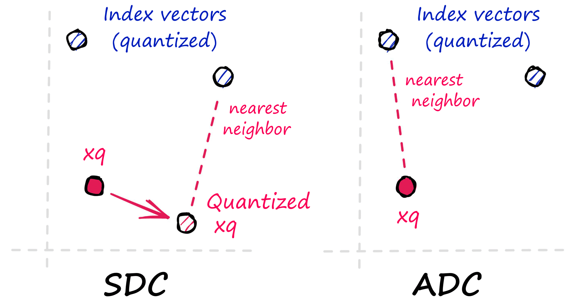
With symmetric distance computation (SDC, left) we quantize xq before comparing it to our previously quantized xb vectors. ADC (right) skips the quantization of xq and compares it directly to the quantized xb vectors.
To implement the index using the index_factory we can write:
In[40]:
index = faiss.index_factory(d, "IVF256,PQ32x8")
index.train(xb)
index.add(xb)
D, I = index.search(xq, k)
recall(I)
With this, we create an IVFADC index with 256 IVF cells; each vector is compressed with PQ using m and nbits values of 32 and 8, respectively. PQ uses nbits == 8 by default so we can also write "IVF256,PQ32".
m: number of subvectors that original vectors are split into
nbits: number of bits used by each subquantizer, we can calculate the number of centroids used by each subquantizer as 2**nbits
We can decrease nbits to reduce index memory usage or increase to improve recall and search speed. However, the current version of Faiss does restrict nbits to >= 8 for IVF,PQ.
It is also possible to increase the index.nprobe value to search more IVF cells — by default, this value is 1.
In[42]:
index.nprobe = 8
D, I = index.search(xq, k)
recall(I)
Here we have our index performance for various nbits and nprobe values:
| Index | nprobe | Recall | Search Time | Memory |
|---|---|---|---|---|
| IVF256,PQ32x4 | 1 | 27% | 329µs | 25MB |
| IVF256,PQ32x4 | 6 | 45% | 975µs | 25MB |
| IVF256,PQ32x8 | 1 | 30% | 136µs | 40MB |
| IVF256,PQ32x8 | 8 | 74% | 729µs | 40MB |
Optimized Product Quantization
IVFADC and other indexes using PQ can benefit from Optimized Product Quantization (OPQ).
OPQ works by rotating vectors to flatten the distribution of values across the subvectors used in PQ. This is particularly beneficial for unbalanced vectors with uneven data distributions.
In Faiss, we add OPQ as a pre-processing step. For IVFADC, the OPQ index string looks like " OPQ32,IVF256,PQ32" where the 32 in OPQ32 and PQ32 refers to the number of bytes m in the PQ generated codes.
The OPQ matrix in Faiss is not the whole rotation and PQ process. It is only the rotation. A PQ step must be included downstream for OPQ to be implemented.
As before, we will need to train the index on initialization.
In[45]:
# we can add pre-processing vector rotation to
# improve distribution for the PQ step using OPQ
index = faiss.index_factory(d, "OPQ32,IVF256,PQ32x8")
index.train(xb)
index.add(xb)
D, I = index.search(xq, k)
recall(I)
In[46]:
%%timeit
index.search(xq, k)
Out[46]:
142 µs ± 2.25 µs per loop (mean ± std. dev. of 7 runs, 10000 loops each)
The data distribution of the Sift1M dataset is already well balanced, so OPQ gives us only a minor increase in recall performance. With an nprobe == 1 we have increased recall from 30% -> 31%.
We can increase our nprobe value to improve recall (at the cost of speed). However, because we added a pre-processing step to our index, we cannot access nprobe directly with index.nprobe as this index no longer refers to the IVF portion of our index.
Instead, we must extract the IVF index before modifying the nprobe value — we can do this using the extract_index_ivf function.
In[47]:
ivf = faiss.extract_index_ivf(index)
ivf.nprobe = 13
D, I = index.search(xq, k)
recall(I)
In[48]:
%%timeit
index.search(xq, k)
Out[48]:
1.08 ms ± 21.1 µs per loop (mean ± std. dev. of 7 runs, 1000 loops each)
With a higher nprobe value of 14 — we return a recall of 74%. A similar recall result to PQ alone, alongside an increased search time from 729µs -> 1060µs.
| Index | nprobe | Recall | Search Time | Memory |
|---|---|---|---|---|
| IVF256,PQ32x4 | 1 | 30% | 136µs | 40.2MB |
| IVF256,PQ32x4 | 1 | 31% | 143µs | 40.3MB |
| IVF256,PQ32x8 | 8 | 74% | 729µs | 40.2MB |
| IVF256,PQ32x8 | 13 | 74% | 1060µs | 40.3MB |
We will see later in the article that OPQ can be used to improve performance, but as we can see here, that is not always the case.
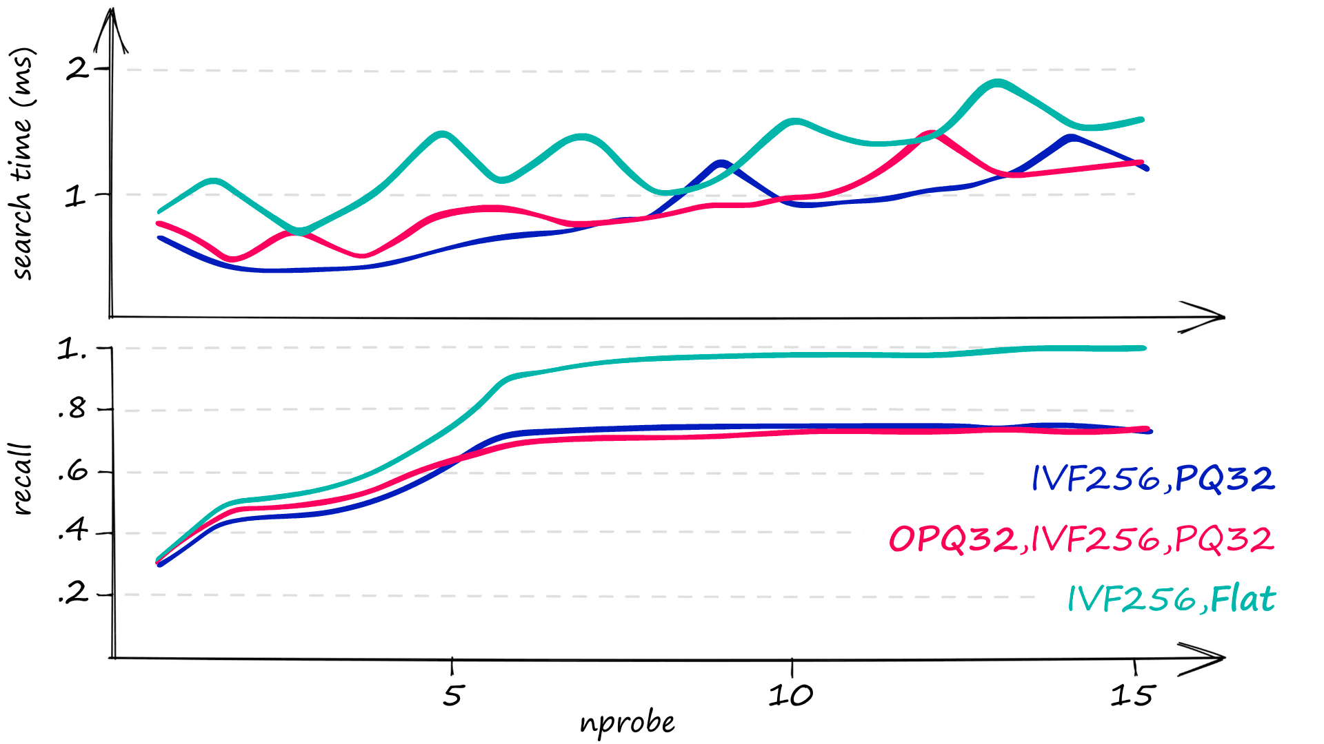
Search time (top) and recall (bottom) for various nprobe values. We have included "IVF256,Flat" for comparison. The flat index has much higher memory usage at 520MB.
OPQ can also be used to reduce the dimensionality of our vectors in this pre-processing step. This dimensionality D must be a multiple of M, preferably D == 4M. To reduce dimensionality to 64, we could use "OPQ16_64,IVF256,PQ16".
Multi-D-ADC
Multi-D-ADC refers to multi-dimensional indexing, alongside a PQ step which produces an asymmetric distance computation at search time (as we discussed previously) [5].
The multi-D-ADC index is based on the inverted multi-index (IMI), an extension of IVF.
IMI can outperform IVF in both recall and search speed but does increase memory usage [7]. This makes IMI indexes (such as multi-D-ADC) ideal in cases where IVFADC doesn’t quite reach the recall and speed required, and you can spare more memory usage. The IMI index works in a very similar way to IVF, but Voronoi cells are split across vector dimensions. What this produces is akin to a multi-level Voronoi cell structure.
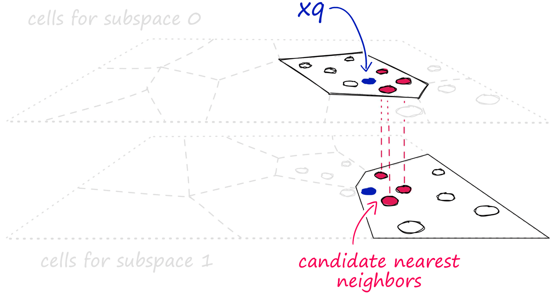
Voronoi cells split across multiple vector subspaces. Given a query vector xq, we would compare each xq subvector to its respective subspace cells.
When we add a vector compression to IMI using PQ, we produce the multi-D-ADC index. Where ADC refers to the asymmetric distance computation that is made when comparing query vectors to PQ vectors.
Putting all of this together, we can create a multi-D-ADC index using the index factory string " IMI2x8,PQ32".
In[50]:
index = faiss.index_factory(d, "IMI2x8,PQ32")
index.train(xb)  # index construction time is large for IMI
index.add(xb)
In[53]:
imi = faiss.extract_index_ivf(index)  # access nprobe
imi.nprobe = 620
D, I = index.search(xq, k)
recall(I)
In[54]:
%%timeit
index.search(xq, k)
Out[54]:
1.35 ms ± 60.2 µs per loop (mean ± std. dev. of 7 runs, 1000 loops each)
To return a similar recall to our IVFADC equivalent, we increased search time to 1.3ms, which is very slow. However, if we add OPQ to our index, we will return much better results.
In[56]:
index = faiss.index_factory(d, "OPQ32,IMI2x8,PQ32")  # lets try with OPQ
index.train(xb)  # index construction time is even larger for OPQ,IMI
index.add(xb)
In[59]:
imi = faiss.extract_index_ivf(index)  # we increase nprobe
imi.nprobe = 100
D, I = index.search(xq, k)
recall(I)
In[60]:
%%timeit
index.search(xq, k)
Out[60]:
461 µs ± 30 µs per loop (mean ± std. dev. of 7 runs, 1000 loops each)
For a recall of 74%, our OPQ multi-D-ADC index is fastest at an average search time of just 461µs.
| Index | Recall | Search Time | Memory |
|---|---|---|---|
| IVF256,PQ32 | 74% | 729µs | 40.2MB |
| IMI2x8,PQ32 | 72% | 1350µs | 40.8MB |
| OPQ32,IMI2x8,PQ32 | 74% | 461µs | 40.7MB |
As before, we can fine-tune the index to prioritize recall or speed using nprobe.
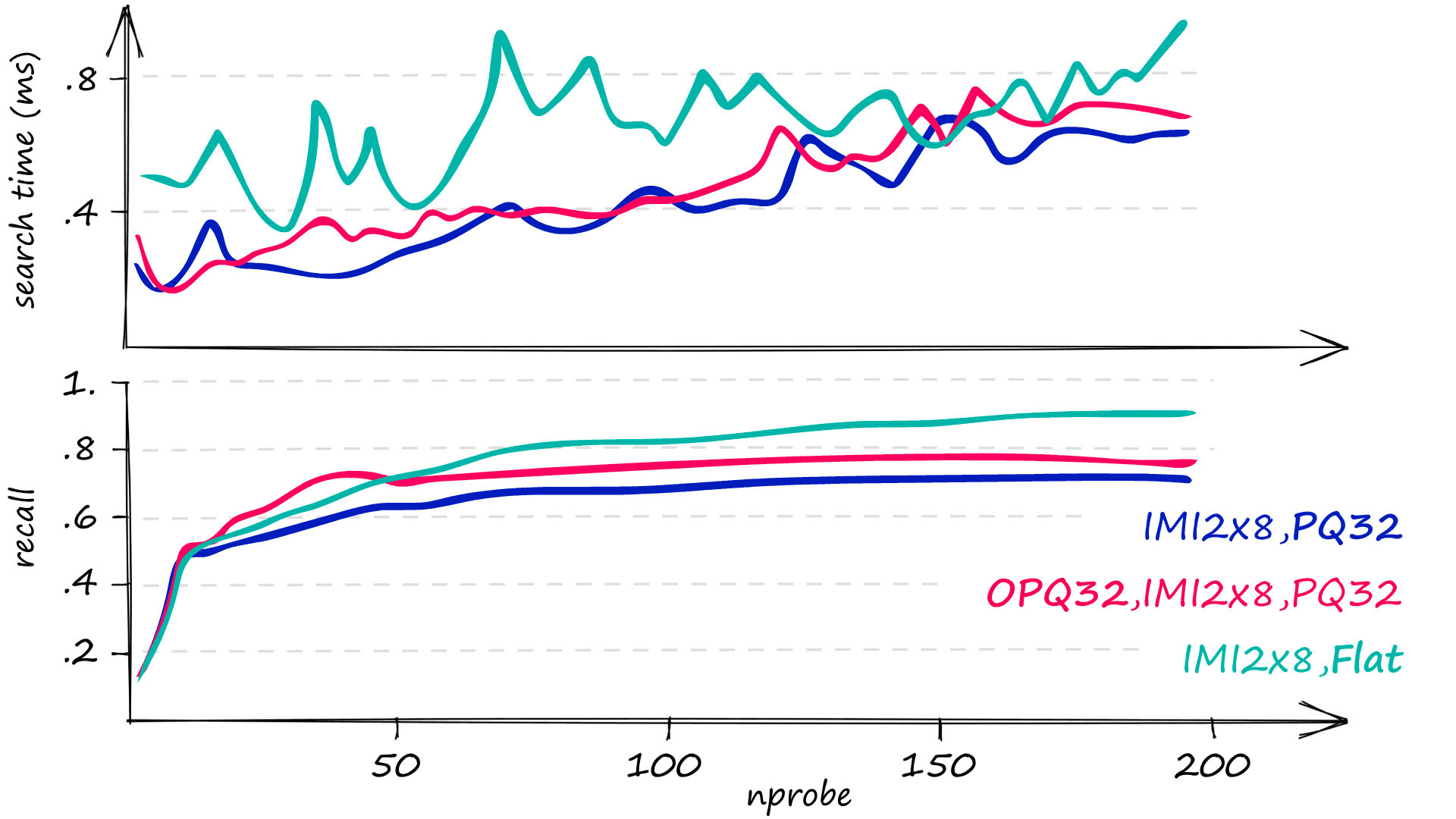
Search time (top) and recall (bottom) for various nprobe values. We have included "IMI2x8,Flat" for comparison. The flat index has much higher memory usage at 520MB.
"OPQ32,IMI2x8,PQ32" is one of our best indexes in terms of recall and speed at low memory. However, we’ll see that we can improve these metrics even further with the following index.
HNSW Indexes
IVF with Hierarchical Navigable Small-World (HNSW) graphs is our final composite index. This index splits our indexed vectors into cells as per usual with IVF, but this time we will optimize the process using HNSW.
Compared to our previous two indexes, IVF with HNSW produces comparable or better speed and significantly higher recall — at the cost of much higher memory usage.
At a high level, HNSW is based on the small-world graph theory that all vertices (nodes) in a network — no matter how large — can be traversed in a small number of steps.
Example of a navigable small-world graph, all nodes within the graph are connected by a small number of edge traversals. Small world graph theory assumes the same to be true even for huge networks with billions of vertices.
In this small world graph, we see both short-range and long-range links. When traversing across long-range links, we move more quickly across the graph.
HNSW takes advantage of this by splitting graph links into multiple layers. At the higher entry layers, we find only long-range links. As we move down the layers, shorter-range links are added.
When searching, we start at these higher layers with long-range links. Meaning our first traversals are across long-range links. As we move down the layers, our search becomes finer as we traverse across more short-range links.
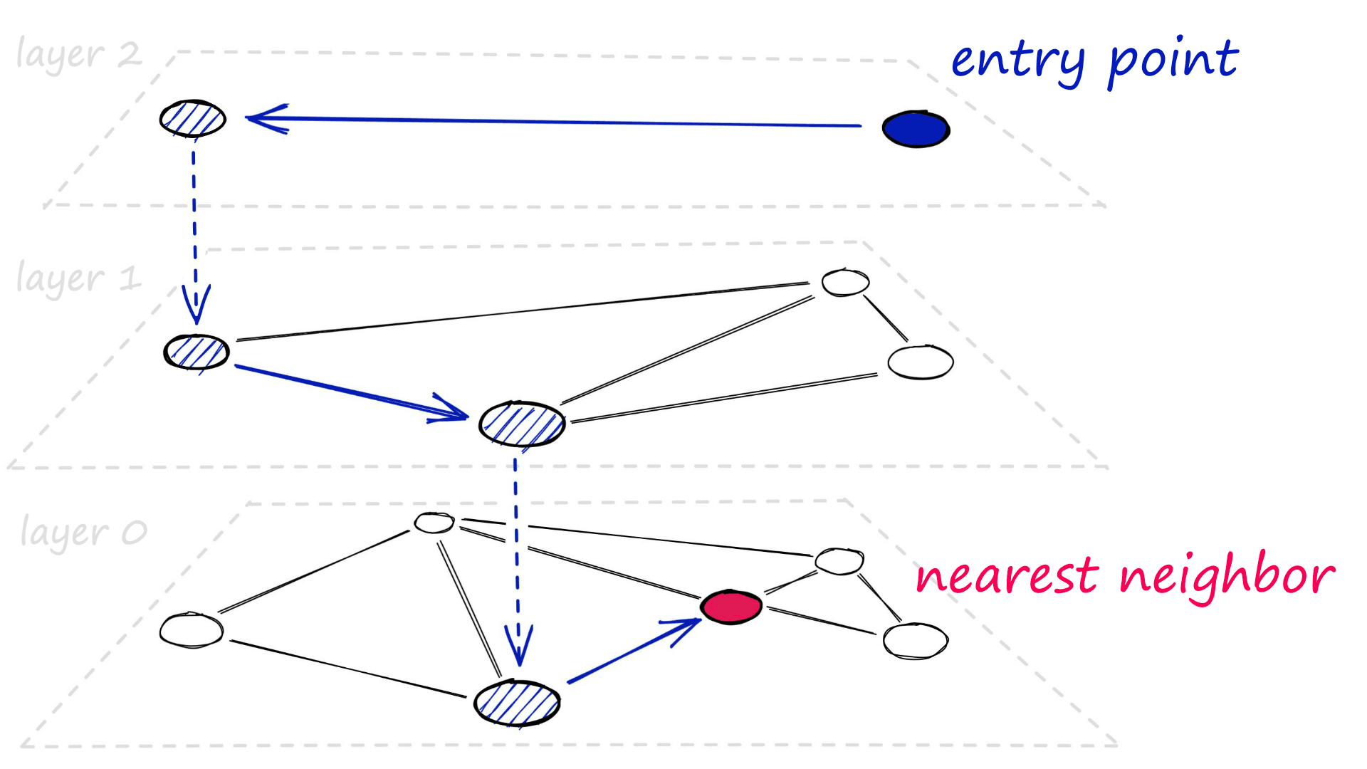
HNSW graphs break the typical graph containing both long-range and short-range links into multiple layers (hierarchies). During the search, we begin at the highest layer, which consists of long-range links. As we move down through each layer, the links become more granular.
This approach should minimize the number of traversals (speeding up search) while still performing a very fine search in the lower layers (maintaining high recall).
That is HNSW, but how can we merge HNSW with IVF?
Using vanilla IVF, we introduce our query vector and compare it to every cell centroid, identifying the nearest centroids for restricting our search scope.
To pair this process with HNSW, we produce an HNSW graph of all of these cell centroids, making the exhaustive centroid search approximate.
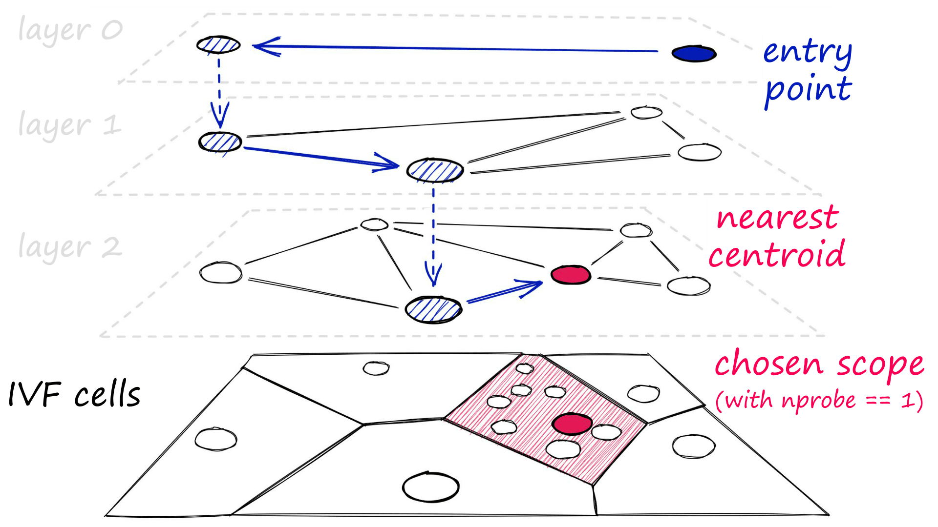
HNSW can be used to quickly find the approximate nearest neighbor using IVF cell centroids.
Previously, we have been using IVF indexes with 256 cell centroids. An exhaustive search of 256 is fast, and there is no reason to use an approximate search with so few centroids.
And because we have so few cells, each cell must contain many vectors - which will still be searched using an exhaustive search. In this case, IVF+HNSW on the cell centroids does not help.
With IVF+HNSW indexes, we need to swap ' few centroids and large cells' for ' many centroids and small cells'.
For our 1M index, an nlist value of 65536 is recommended [8]. However, we should provide at least 30*nlist == 1.97M vectors to index.train, which we do not have. So a smaller nlist of 16384 or less is more suitable. For this dataset, nlist == 4096 returned the highest recall (at slower speeds).
Using IVF+HNSW, we quickly identify the approximate nearest cell centroids using HNSW, then restrict our exhaustive search to those nearest cells.
The standard IVF+HNSW index can be built with "IVF4096_HNSW32,Flat". Using this, we have:
4096IVF cells.- Cell centroids are stored in an HNSW graph. Each centroid is linked to
32other centroids. - The vectors themselves have not been changed. They are
Flatvectors.
In[62]:
index = faiss.index_factory(d, "IVF4096_HNSW32,Flat")
index.train(xb)
index.add(xb)
In[63]:
D, I = index.search(xq, k)
recall(I)
In[64]:
%%timeit
index.search(xq, k)
Out[64]:
58.9 µs ± 3.25 µs per loop (mean ± std. dev. of 7 runs, 10000 loops each)
In[65]:
index.nprobe = 146
D, I = index.search(xq, k)
recall(I)
In[66]:
%%timeit
index.search(xq, k)
Out[66]:
916 µs ± 9.23 µs per loop (mean ± std. dev. of 7 runs, 1000 loops each)
With this index, we can produce incredible performance ranging from 25% -> 100% recall at search times of 58.9µs -> 916µs.
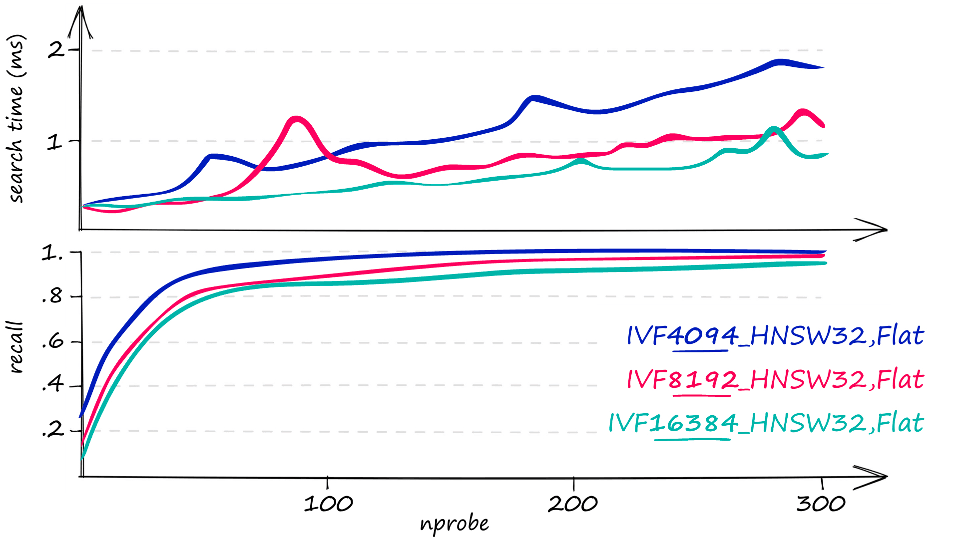
Search time (top) and recall (bottom) for various nprobe values. At the cost of longer search times, we can increase recall by decreasing nlist.
However, the IVF+HNSW index is not without its flaws. Although we have incredible recall and fast search speeds, the memory usage of this index is huge. Our 1M 128-dimensional vectors produce an index size of 523MB+.
As we have done before, we can reduce this using PQ and OPQ, but this will reduce recall and increase search times.
| Index | Recall | Search Time | Memory |
|---|---|---|---|
| IVF4096_HNSW,Flat | 90% | 550µs | 523MB |
| IVF4096_HNSW,PQ32 (PQ) | 69% | 550µs | 43MB |
| OPQ32,IVF4096_HNSW,PQ32 (OPQ) | 74% | 364µs | 43MB |
If a lower recall is acceptable for minimizing search time and memory usage, the IVF+HNSW index with OPQ is ideal. On the other hand, IVF+HNSW with PQ offers no benefit over our previous IVFADC and Multi-D-ADC indexes.
| Name | Index String | Recall | Search Time | Memory |
|---|---|---|---|---|
| IVFADC | IVF256,PQ32 | 74% | 729µs | 40MB |
| Multi-D-ADC | OPQ32,IMI2x8,PQ32 | 74% | 461µs | 41MB |
That’s it for this article! We introduced composite indexes and how to build them using the Faiss index_factory. We explored several of the most popular composite indexes, including:
- IVFADC
- Multi-D-ADC
- IVF-HNSW
By indexing and searching the Sift1M dataset, we learned how to modify each index’s parameters to prioritize recall, speed, and memory usage.
With what we have covered here, you will be able to design and test a variety of composite indexes and better decide on an index structure that best suits your needs.
References
[1] Y.Chen, et al., Approximate Nearest Neighbor Search by Residual Vector Quantization (2010), Sensors
[2] Y. Matsui, et al., A Survey of Product Quantization (2018), ITE Trans. on MTA
[3] T. Ge, et. al., Optimized Product Quantization (2014), TPAMI
[4] H. Jégou, et al., Product quantization for nearest neighbor search (2010), TPAMI
[5] A. Babenko, V. Lempitsky, The Inverted Multi-Index (2012), CVPR
[6] H. Jégou, et al., Searching in One Billion Vectors: Re-rank with Source Coding (2011), ICASSP
[7] D. Baranchuk, et al., Revisiting the Inverted Indices for Billion-Scale Approximate Nearest Neighbors (2018), ECCV
[8] Guidelines to choose an index, Faiss wiki
[9] The Index Factory, Faiss wiki
Was this article helpful?