





One of the most frequently asked questions we get at Pinecone is: “How do I semantically search over structured (or semi-structured) data?”
Our answer almost always is: “Well, it depends…”
If you’re a decision maker in charge of figuring out whether to put your semi-/structured data into a vector database, you should ask yourself the following questions:
If your answer to both is yes, you should consider vectorizing your data and storing it in a vector DB. If your answer to both was no, remember, always use the right tool for the right job.
This post will:
→ If you are mostly here to snag some code snippets for vectorizing tabular data, feel free to jump right into the demo notebook.
Figuring out whether your data will benefit from vector search (i.e. semantic search) is not always straightforward. Below are some tips to help you arrive at an answer.
Some use cases where you should not index semi-/structured data in a vector DB:
On the other hand, the following are use cases where running semantic searches over semi-/structured data can produce valuable results:
Before diving into different strategies you can use to vectorize semi-/structured data, let’s get on the same page about different data types and concepts.
Structured data
Structured data is pretty much anything that has a predefined schema. Examples of structured data are CSV files, tables, or spreadsheets.
→ This is the kind of data we’ll be experimenting with later!
Unstructured data
Unstructured data is nearly always natural language-based (whether in audio or text format). You can think of things like Reddit comments, essays, recorded Zoom conversations, etc. The need to understand this type of data is what spurred the invention of vector search in the first place – vectors allow people to understand the latent semantic meaning(s) of unstructured data.
Semi-structured data
Semi-structured data refers to data that is “self-describing.” Examples are JSON or XML files. These types of files contain structural information about the data they represent. Semi-structured data has constructs such as hierarchies, which are created by nested semantic elements, e.g. metadata tags. Semi-structured data can also easily evolve over time, since it lacks a fixed schema.
Hybrid search
Many people confuse the concept of semantically searching over structured data with the concept of hybrid search. While the two ideas might sound similar, semantically searching over structured and unstructured data (i.e. what we do in this post) is different from combining semantic search with keyword search (i.e. hybrid search).
When we say “hybrid search,” we are referring to conducting a semantic search over “dense” vectors in addition to also conducting a keyword search over “sparse” vectors. Dense vectors are semantic representations of data created by embedding models, while sparse vectors are essentially vectorized inverted indexes, such as those created by algorithms like BM25 and TF-IDF.
You can conduct a hybrid search over structured, unstructured, or semi-structured data.
This post is not about hybrid search.
Much of the data sitting in data warehouses today is structured or semi-structured. Figuring out the best way to semantically search over this content is often not straightforward. You also don’t always need to resort to vectorization in order to work with semi-/structured data in a semantic search context. Below is a cursory overview of some popular non-vector methods we’ve seen in the field.
Non-vector techniques
If you’ve already extracted some well-formed semi-/structured data from a source, there are many ways to map that structure to vector space. Some strategies we have seen include:
The above are all valid methods, and some (e.g. using prefix IDs and/or metadata payloads) are often lower lifts than vectorizing your semi-/structured data. Depending on your use case, a non-vector strategy might work best.
In this post, though, we’ll be looking at vectorization strategies, specifically. Comparing four different methods, we’ll aim to figure out which popular vectorization strategy nets us the most relevant search results when asking an LLM questions about a research article with embedded tables.
The meat of this post is an experiment that compares the results of different vectorization techniques in the context of a RAG (Retrieval-Augmented Generation) application. The vectorization methods in the experiment are all real strategies we at Pinecone have seen customers implement.
Note: while the following experiment does not include the non-vector techniques mentioned above, it is fairly common to combine vector and non-vector methods to get even more relevant results.
For this experiment, you will use Unstructured and LangChain to extract tables from a PDF. You will then use LlamaIndex and Pinecone to extract the remaining, non-table PDF contents; vectorize and store all the extracted data; and finally query the vectors within a RAG application.
See this notebook for the full code implementation; what follows is an overview.
You will evaluate how a RAG application’s answers to 7 questions change depending on the vectorization technique applied to two of the tables extracted from the PDF.
The two tables you will use represent different experimentation results from a research paper on neural rankers.
Table 1 looks like this:
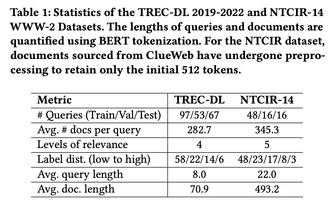
Table 1
Table 2 looks like this:
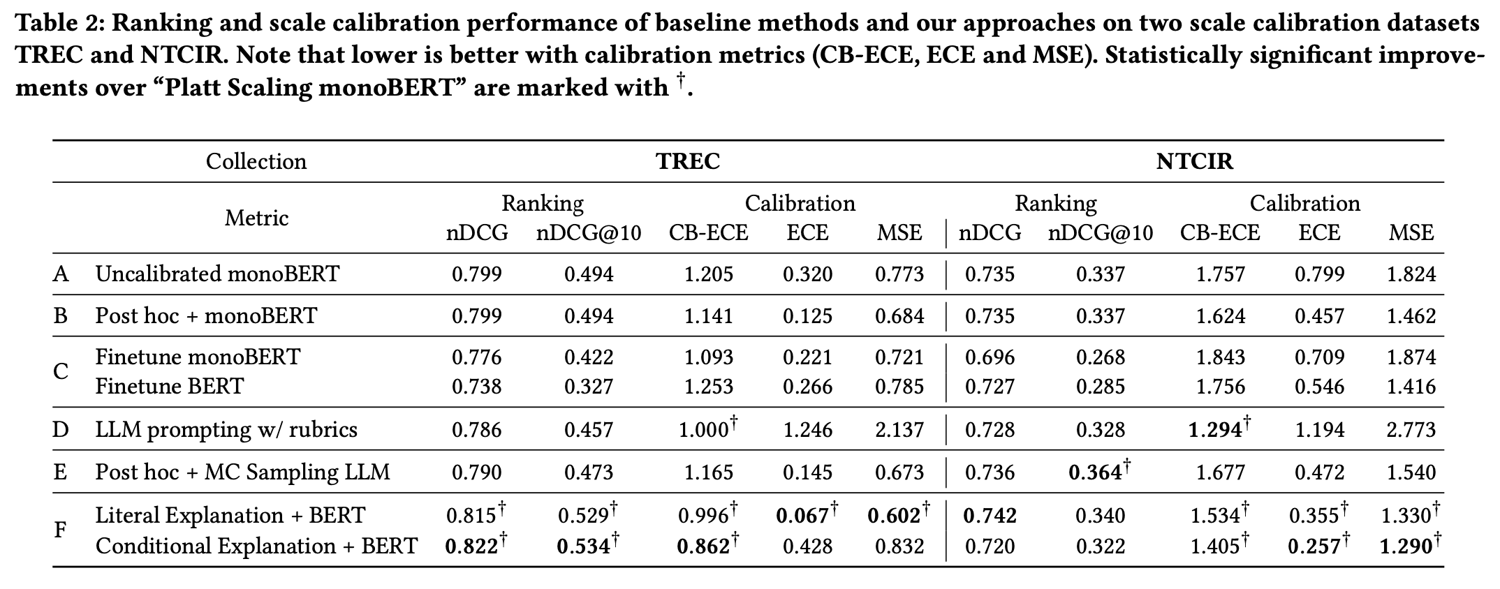
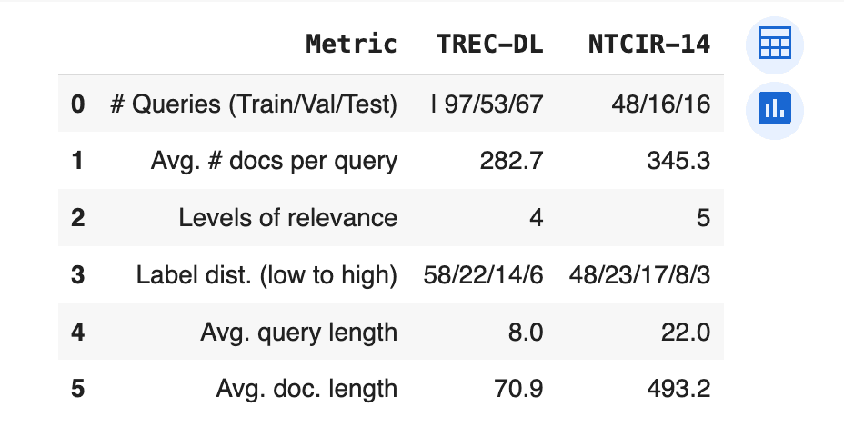
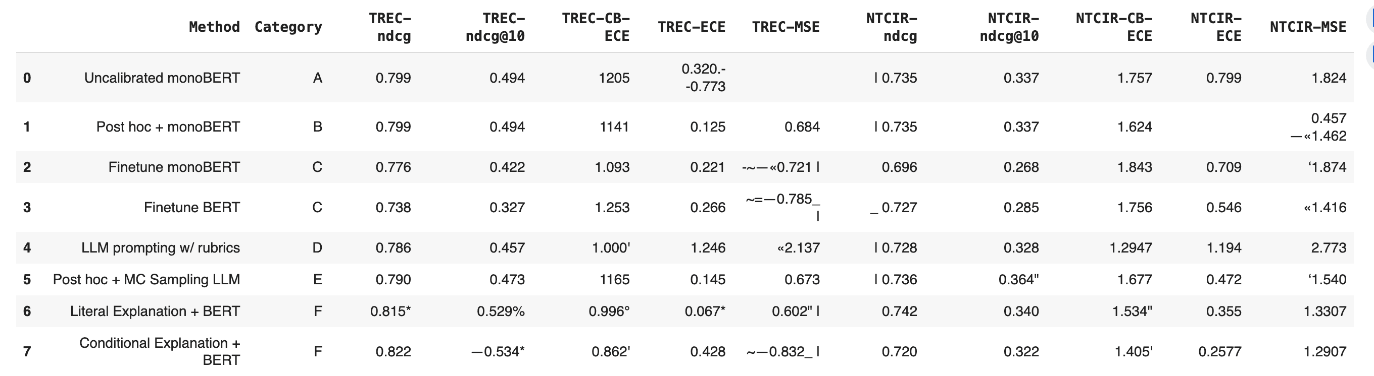
You will turn the extracted table elements into two dataframes, called df1 and df2, respectively.
Note: the ways in which these dataframes are laid out are up to you – the concatenation of certain header columns, etc. are strategic choices we made based on what data we identified as having the most semantic value.
df1 looks like this:
df1
df2 looks like this:
df2
You will run the same 7 questions through each variants’ RAG pipeline to compare LLM outputs. The questions and their (ideal) answers are below.
You will run five different scenarios to ascertain the impact of different vectorization strategies on table elements:
control variant, you will process the entire PDF file, paying no particular attention to whether it has tables or any other embedded structures of interest.A control document looks like this:

Preview of control document
variant 1, you will concatenate all the values per row into a single string (and, ultimately, vector), per table. As shown below for df2, each row contains the name of the strategy, its category, and its scores.
Preview of variant 1 row
variant 1, for variant 2 you will take the concatenated row data and to each row add the column header (per table). Df2 sample shown below:
Preview of variant 2 row
Variant 3 will be the same as variant 2, with the addition of each table’s description, e.g.:
Preview of variant 3 row
df2, each row has been turned into a natural language phrase, representing the row’s data:
Preview of variant 4 row
Vector DB
You will run your experiments on a Pinecone serverless index, using cosine similarity as your similarity metric and AWS as your cloud provider.
ML Models
Through Unstructured, you will use the Yolox model for identifying and extracting the embedded tables from the PDF.
Later, you will use LlamaIndex to build a RAG pipeline that uses two OpenAI models: ada-002, an embedding model, for semantically chunking up your data and creating your text embeddings; and gpt-3.5-turbo, an LLM, for answering the questions.
Overview of RAG Pipeline
This is what your RAG pipeline looks like:
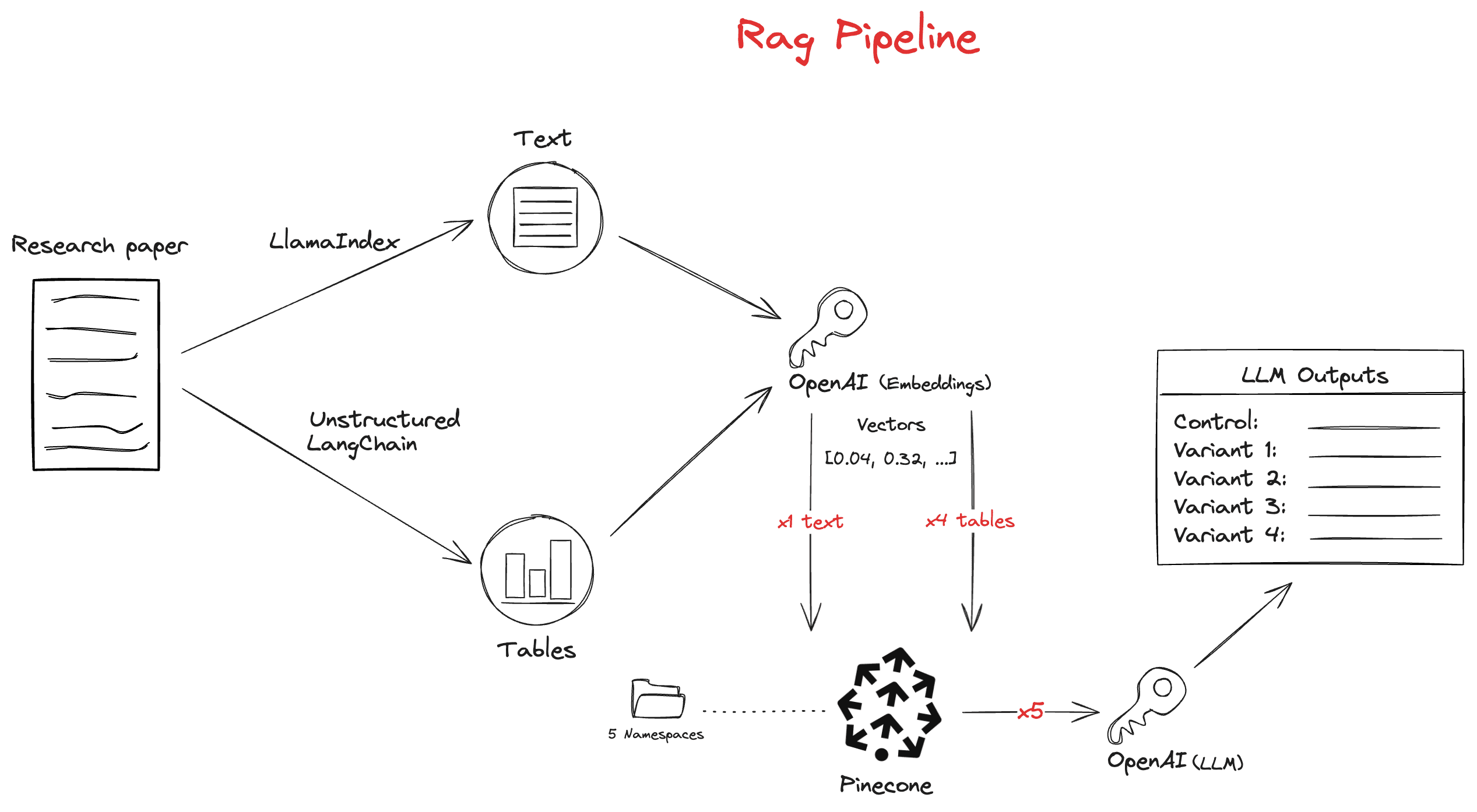
Overview of RAG pipeline in experiment
For the experiment’s use case (RAG chatbot over a research article), the vectorization strategy that provides the most accurate answers across the most questions is…it depends 🫠!
From a bird’s eye view, the most “successful” methods was concatenating row data with other data, as in variants 2 and 3.
But, of course, it’s not that simple…
| Variant | Correct | Incorrect |
|---|---|---|
| control | 6 | 1 |
| v1: concatenating rows | 6 | 1 |
| v2: concatenating rows, headers | 7 | 0 |
| v3: concatenating rows, headers, table descriptions | 7 | 0 |
| v4: injecting table values into natural language phrase(s) | 6 | 1 |
| Questions | Control | V1 | V2 | V3 | V4 |
|---|---|---|---|---|---|
| Q1 | Correct | Correct | Correct | Correct | Correct |
| Q2 | Incorrect | Incorrect | Correct | Correct | Correct |
| Q3 | Correct | Correct | Correct | Correct | Correct |
| Q4 | Correct | Correct | Correct | Correct | Correct |
| Q5 | Correct | Correct | Correct | Correct | Correct |
| Q6 | Correct | Correct | Correct | Correct | Correct |
| Q7 | Correct | Correct | Correct | Correct | Incorrect |
The question the majority of variants got incorrect was question 2: “What are the Literal Explanation + BERT method's ndcg@10 scores on both datasets in table 2?” What is it about this question that tripped up the LLM?
If you compare question 2 to the other questions, there is one thing that stands out: question 2 is the only question whose correct answer would be a quantity(ies) from a row within a table.
The variants that got this question wrong were the control variant and v1, v2 (the concatenated rows and headers), v3 (v2’s data plus each table’s description), and v4, (the natural language phrase), got question 2 right. It’s notable that these variants represented the most invasive vectorization methods.
For v2, the relevant row sent to the LLM looked like this:
Method: Literal Explanation + BERT, Category: F, TREC-ndcg: 0.815*, TREC-ndcg@10: 0.529%, TREC-CB-ECE: 0.996°, TREC-ECE: 0.067*, TREC-MSE: 0.602" |, NTCIR-ndcg: 0.742, NTCIR-ndcg@10: 0.340, NTCIR-CB-ECE: 1.534", NTCIR-ECE: 0.355, NTCIR-MSE: 1.3307
For v3, it looked like this:
Method: Literal Explanation + BERT, Category: F, TREC-ndcg: 0.815*, TREC-ndcg@10: 0.529%, TREC-CB-ECE: 0.996°, TREC-ECE: 0.067*, TREC-MSE: 0.602" |, NTCIR-ndcg: 0.742, NTCIR-ndcg@10: 0.340, NTCIR-CB-ECE: 1.534", NTCIR-ECE: 0.355, NTCIR-MSE: 1.3307. Table 2: Ranking and scale calibration performance of baseline methods and our approaches on two scale calibration datasets\nTREC and NTCIR. Note that lower is better with calibration metrics (CB-ECE, ECE and MSE). Statistically significant improve-\nments over “Platt Scaling monoBERT” are marked with
And for v4, it looked like this:
Against the TREC dataset, the "Literal Explanation + BERT" method (from the "F" category) got a nDCG score of 0.815*, a nDCG@10 score of 0.529%, a CB-ECE score of 0.996°, an ECE score of 0.067*, and an MSE score of 0.602" |. Against the NTCIR dataset, the "Literal Explanation + BERT" method (from the "F" category) got a nDCG score of 0.742, a nDCG@10 score of 0.340, a CB-ECE score of 1.534", an ECE score of 0.355, and an MSE score of 1.3307.
In comparison, the control looked like this:
\nFLiteral Explanation + BERT 0.815†0.529†0.996†0.067†0.602†0.742 0.340 1.534†0.355†1.330†\n
You can see there is hardly any semantic information contained in the control. It makes sense that the vectorization methods in which we artificially injected the most semantic information were the winners.
Takeaway 1: to semantically search over quantitative, tabular data, your best bet is to wrap the data in as much semantic information as possible.
Most of the other questions demand some type of semantic extrapolation in order to be answered (e.g. ‘compare this and that’, ‘tell me how to interpret something’, ‘does this word mean the same thing as this word?’). When it comes to these types of questions, the results show that the LLM (gpt-3.5-turbo) is pretty good at answering correctly no matter what human intervention is taken (or not taken).
Within these correct answers, though, there are some more-helpful and less-helpful answers.
Take, for instance, question 4: “How do I interpret table 2's calibration and ranking scores?”
Control answer:
Interpreting Table 2's calibration and ranking scores involves looking at the metrics provided for different approaches on two datasets, TREC and NTCIR. The metrics include nDCG (normalized discounted cumulative gain), nDCG@10 (nDCG at the top 10 results), CB-ECE (class-balanced expected calibration error), ECE (expected calibration error), and MSE (mean square error). Lower values are better for calibration metrics like CB-ECE, ECE, and MSE. Statistically significant improvements over a specific baseline method are marked with a dagger symbol (†). By comparing the values of these metrics across different approaches in the table, one can assess the performance of each method in terms of both ranking and calibration on the specified datasets.
V2 answer:
Interpret the calibration and ranking scores in Table 2 by considering that lower values are better for calibration metrics such as CB-ECE, ECE, and MSE. Look for statistically significant improvements over the "Platt Scaling monoBERT" method, which are marked with a dagger symbol (†). Pay attention to the values in the table for different methods and metrics, comparing them to understand the performance of each approach in terms of both ranking and calibration on the TREC and NTCIR datasets.
You can see that the control’s answer is more explanatory and verbose than variant 2’s answer, expanding and defining each acronym and telling the user how to assess performance. The control’s answer is demonstrably more helpful (unless your business logic deems that answer is too rudimentary).
The control variant’s answers being exceedingly helpful is a trend across the rest of the questions.
Takeaway 2: for answering general, semantic questions that may or may not rely on structured data, your best bet is to simply do nothing (at first).
Arguably, doing nothing is the most scalable approach mentioned. Simply extract your text data and your structured data, squish it altogether, feed it to an LLM, and see what happens. Doing nothing is also evidently one of the best strategies, too!
Only if your LLM’s answers are unsatisfactory, should you then take a more heavy-handed approach. Anecdotally from us at Pinecone (and as supported by the experiment), concatenating row values with their header data is a great place to start.
We’d love to hear what you’ve done when it comes to searching over semi-/structured data. Reach out!
此内容由惯性聚合(RSS阅读器)自动聚合整理,仅供阅读参考。 原文来自 — 版权归原作者所有。