







Vector similarity search makes massive datasets searchable in fractions of a second. Yet despite the brilliance and utility of this technology, often what seem to be the most straightforward problems are the most difficult to solve. Such as filtering.
Filtering takes the top place in being seemingly simple — but actually incredibly complex. Applying fast-but-accurate filters when performing a vector search (ie, nearest-neighbor search) on massive datasets is a surprisingly stubborn problem.
This article explains the two common methods for adding filters to vector search, and their serious limitations. Then we will explore Pinecone’s solution to filtering in vector search.
In vector similarity search we build vector representations of some data (images, text, cooking recipes, etc), storing it in an index (a database for vectors), and then searching through that index with another query vector.
If you found this article through Google, what brought you here was a semantic search identifying that the vector representation of your search query aligned with Google’s vector representation of this page.
Netflix, Amazon, Spotify, and many others use vector similarity search to power their recommendation systems, using it to identify similar users and base their new show, product, or music recommendations on what these similar groups of people seem to like.
In search and recommender systems there is almost always a need to apply filters: Google can filter searches by category (like news or shopping) , date, or even language and region; Netflix, Amazon, and Spotify may want to focus on comparing users in similar geographies. Restricting the search scope to relevant vectors is — for many use-cases — an absolute necessity for providing a better customer experience.
Despite the clear need, there has been no good approach for metadata filtering — restricting the scope of a vector search based on a set of metadata conditions — that’s both accurate and fast.
We may want to restrict our search to a category of records or a specific date range.
For example, say we want to build a semantic search application for a large corporation to search through internal documents. Users will often want to filter their search to a specific department. It should be as simple as writing this pseudo-code:
top-k where department == 'engineering'
OR
top-k where department != 'hr'

top-k where {“department”: {"$eq": "engineering"}}
OR
top-k where {“department”: {"$ne": "hr"}}
And what if we only want the last few weeks of data? Or need to see how the documents have changed over time — we would want to restrict the search to old records only!
top-k where date >= 14 days ago
OR
top-k where date < 3 years ago

top-k where {“date”: {"$gte": 14}}
OR
top-k where {“date”: {"$lt": 1095}}
There are countless variations and combinations of queries just like these.
top-k where date >= 14 days ago AND department == 'finance'

top-k where {"date": {"$gte": 14}, “department”: {"$eq": "finance"}}
Without filters, we restrict our ability to build powerful tools for search. Imagine Excel without data filters, SQL without a WHERE clause, or Python without if...else statements. The capabilities of these tools become massively diminished, and the same applies to vector search without filters.
But implementing such filters into a semantic/vector search application isn’t easy. Let’s first look at the two most common approaches — along with their advantages and disadvantages. They are pre-filtering and post-filtering.
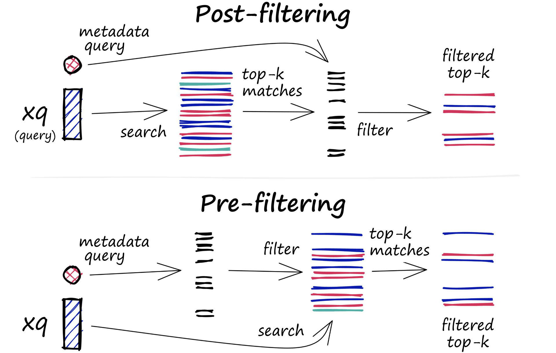
These approaches require two indexes: The vector index as per usual, and a metadata index. It is through this metadata index that we identify those vectors which satisfy our filter conditions.
The first approach we could take is to pre-filter our vectors. This consists of taking our metadata index and applying our set of conditions. From here, we return a list of all records in our vector index that satisfies our filter conditions.
Now when we search, we’ve restricted our scope — so our vector similarity search will be faster, and we’ll only return relevant results!
The problem is that our pre-filter disrupts how ANN engines work (ANN requires the full index), leaving us with two options:
Build an ANN index for every possible filter. Perform a brute-force kNN search across remaining vectors.
Option (1) is simply not practical, there are far too many possible filter outputs in a typical index.
That leaves us with option (2), creating the additional overhead of brute-force checking every single vector embedding remaining after the metadata filter.
Pre-filtering is excellent for returning relevant results, but significantly slows-down our search due to the exhaustive, brute-force search that’s required.
While slow for smaller datasets — the problem is exacerbated for larger datasets. This brute-force search is simply not manageable for datasets in the millions or billions.
Maybe post-filtering will work better?
We can’t rely on a brute-force search every time we apply a filter, so what if we applied the filter after our vector search?
Working through it, we have our vector index and a query — we perform a similarity search as usual. We return k of the top nearest matches. We’ll set k == 10.
We’ve now got our top 10 best matches, but there’s plenty of vectors in here that would not satisfy our filter conditions.
We go ahead and apply our post-search filter to remove those irrelevant results. That filter has removed six of our results, leaving us with just four results. We wanted ten results, and we’ve returned four. That’s not so great.
Unfortunately, it gets worse… What if we didn’t return any results in the top k that satisfy our filter conditions? That leaves us with no results at all.
By applying our metadata filter post-search, we avoid the speed issues of an initial brute-force search. Still, we risk returning very few or even zero results, even though there may be relevant records in the dataset. So much for improving customer experience…
We can eliminate the risk of returning too few (or zero) results by increasing k to a high number. But now we have slower search times thanks to our excessively high k searches, and so we’re back to the slow search times of pre-filtering.
Slow search with pre-filtering, or unreliable results with post-filtering. Neither of these approaches sounds particularly attractive, so what can we do?
Pinecone’s single-stage filtering produces the accurate results of pre-filtering at even faster speeds than post-filtering.
It works by merging the vector and metadata indexes into a single index — resulting in a single-stage filter as opposed to the two-stage filter-and-search method of pre- and post-filtering.
This gives us pre-filtering accuracy benefits without being restricted to small datasets. It can even increase search speeds whether you have a dataset of 1 million or 100 billion.
Exactly how this works will be covered in a later article. For now, let’s explore some of the new single-stage filtering features and test its performance.
Filtering in Pinecone is effortless to use. All we need are some vectors, metadata, and an API key.
In this example we use the Stanford Question and Answering Dataset (SQuAD) for both English and Italian languages.
The SQuAD datasets are a set of paragraphs, questions, and answers. Each of those paragraphs is sourced from different Wikipedia pages, and the SQuAD data includes the topic title:
{
 'id': '573387acd058e614000b5cb5',
 'title': 'University_of_Notre_Dame',
 'context': 'One of the main driving forces in the growth of the University was its football team, the ... against the New York Giants in New York City.',
 'question': 'In what year did the team lead by Knute Rockne win the Rose Bowl?',
 'answers': {
 'text': '1925',
 'answer_start': 354
 }
}
From this, we have two metadata tags:
lang — the source text’s language (either en or it).title — the topic title of the source text.We pre-process the datasets to create a new format that looks like:
{
 'id': '573387acd058e614000b5cb5en',
 'context': 'One of the main driving forces in the growth of the University was its football team, the ... against the New York Giants in New York City.',
 'metadata': {
 'lang': 'en',
 'title': 'University_of_Notre_Dame'
 }
}
For Pinecone, we need three items: id, vector, and metadata. We have two of those, but we’re missing our vector field.
The vector field will contain the dense vector embedding of the context. We can build these embeddings using models from sentence-transformers.
We will search in either English or Italian in our use case and return the most similar English/Italian paragraphs. For this, we will need to use a multi-lingual vector embedding model. We can use the stsb-xlm-r-multilingual transformer model from sentence-transformers to do this.
Let’s go ahead and encode our context values:
In[12]:
from sentence_transformers import SentenceTransformer
embedder = SentenceTransformer('stsb-xlm-r-multilingual')

dataset = dataset.map(
    lambda x: {
        'vector': embedder.encode(x['context']).tolist()
    }, batched=True, batch_size=16)
Out[12]:
100%|██████████| 2518/2518 [41:24<00:00, 1.01ba/s]
Out[13]:
Dataset({
    features: ['__index_level_0__', 'context', 'id', 'metadata', 'vector'],
    num_rows: 40281
})
The new format we produce includes our sample id, text, vector, and metadata, which we can go ahead and upsert to Pinecone:
{
 'id': '573387acd058e614000b5cb5en',
 'vector': [0.1, 0.8, 0.2, ..., 0.7],
 'metadata': {
 'lang': 'en',
 'title': 'University_of_Notre_Dame'
 }
}
We can add as many metadata tags as we’d like. They can even contain numerical values.
Now, all we need to do is build our Pinecone index. We can use the Python client — which we install using pip install pinecone.
Using an API key we can initialize a new index for our SQuAD data with:
In[17]:
pinecone.init(
    api_key=key,
    environment='YOUR_ENV'  # find env with API key in console
)
In[19]:
pinecone.create_index(name='squad-test', metric='euclidean', dimension=768)In[20]:
index = pinecone.Index('squad-test')And we’re ready to upsert our data! We’ll perform the upload in batches of 100:
In[21]:
from tqdm.auto import tqdm  # for progress bar

batch_size = 100
for i in tqdm(range(0, len(dataset), batch_size)):
    # set end of current batch
    i_end = i + batch_size
    if i_end > len(dataset):
        # correct if batch is beyond dataset size
        i_end = len(dataset)
    batch = dataset[i: i_end]
    # upsert the batch
    index.upsert(vectors=zip(batch['id'], batch['vector'], batch['metadata']))
Out[21]:
100%|██████████| 403/403 [14:32<00:00, 2.17s/it]
That’s it — our vectors and metadata are ready to go!
Let’s start with an unfiltered search. We’ll search for paragraphs that are similar to "Early engineering courses provided by American Universities in the 1870s". We encode this using the sentence-transformer model, then query our index with index.query.
In[22]:
from sentence_transformers import SentenceTransformer
embedder = SentenceTransformer('stsb-xlm-r-multilingual')

xq = embedder.encode("Early engineering courses provided by American Universities in the 1870s.")
In[23]:
results = index.query(queries=[xq.tolist()], top_k=3)
results
Out[23]:
{'results': [{'matches': [{'id': '5733a6424776f41900660f51it',
                           'score': 106.119217,
                           'values': []},
                          {'id': '56e7906100c9c71400d772d7it',
                           'score': 117.300644,
                           'values': []},
                          {'id': '56e7906100c9c71400d772d7en',
                           'score': 121.347099,
                           'values': []}],
              'namespace': ''}]}
In[24]:
%%timeit
index.query(queries=[xq.tolist()], top_k=3)  # we can compare this search time later
Out[24]:
38.7 ms ± 427 µs per loop (mean ± std. dev. of 7 runs, 10 loops each)
We’re returning the three top_k (most similar) results — Pinecone returns our IDs and their respective similarity scores. As we have our contexts stored locally, we can map these IDs back to our contexts using a dictionary (get_sample) like so:
In[26]:
ids = [i['id'] for i in results['results'][0]['matches']]
ids
Out[26]:
['5733a6424776f41900660f51it',
 '56e7906100c9c71400d772d7it',
 '56e7906100c9c71400d772d7en']
In[27]:
get_sample = {
    x['id']: {
        'context': x['context'],
        'metadata': x['metadata']
    } for x in dataset}
In[28]:
for i in ids:
    print(get_sample[i])
Out[28]:
{
  'context': 'Il Collegio di Ingegneria è stato istituito nel 1920, tuttavia, i primi corsi di ingegneria civile e meccanica sono stati una parte del Collegio di Scienze dal 1870s. Oggi il college, ospitato nella Fitzpatrick, Cushing e Stinson-Remick Halls of Engineering, comprende cinque dipartimenti di studio - ingegneria aerospaziale e meccanica, ingegneria chimica e biomolecolare, ingegneria civile e scienze geologiche, informatica e ingegneria, ingegneria elettronica - con otto B. S lauree offerte. Inoltre, il college offre cinque anni di corsi di laurea doppia con i college of Arts and Letters e di Business Award ulteriore B.',
  'metadata': {'lang': 'it', 'title': ''}
}
{
  'context': 'La KU School of Engineering è una scuola di ingegneria pubblica accreditata ABET situata nel campus principale. La Scuola di Ingegneria è stata ufficialmente fondata nel 1891, anche se i diplomi di ingegneria sono stati rilasciati già nel 1873.',
  'metadata': {'lang': 'it', 'title': ''}
}
{
  'context': 'The KU School of Engineering is an ABET accredited, public engineering school located on the main campus. The School of Engineering was officially founded in 1891, although engineering degrees were awarded as early as 1873.',
  'metadata': {'lang': 'en', 'title': 'University_of_Kansas'}
}
The first Italian paragraph reads:
The College of Engineering was established in the 1920s, however, the first courses in civil and mechanical engineering have been a part of the College of Sciences since the 1870s. Today the college, housed in the Fitzpatrick, Cushing and Stinson-Remick Halls of Engineering, comprises five study departments - aerospace and mechanical engineering, chemical and biomolecular engineering, civil engineering and geological sciences, computer science and engineering, electronic engineering - with eight B. S bachelor's offers. In addition, the college offers five years of dual degree programs with the College of Arts and Letters and an additional B.So we’re getting great results for both English and Italian paragraphs. However, what if we’d prefer to return English results only?
We can do that using Pinecone’s single-stage filtering. Filters can be built using a set of operators that can be applied to strings and/or numbers:
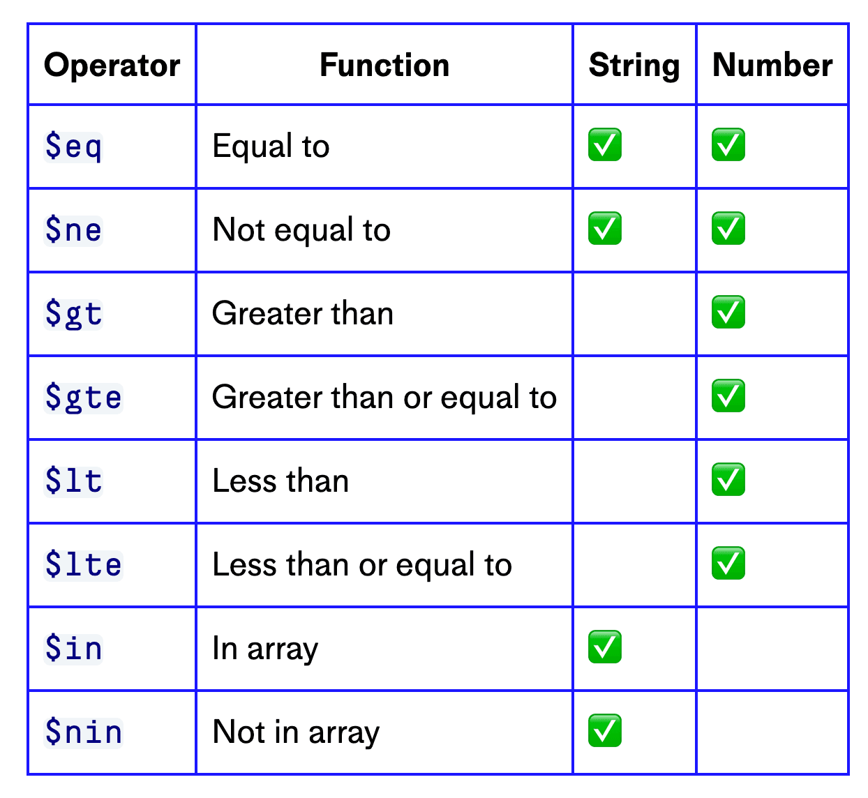
We’re looking to filter based on if lang is equal to ($eq) en. All we do is add this filter condition to our query:
In[29]:
results = index.query(queries=[xq.tolist()], top_k=3, filter={'lang': {'$eq': 'en'}})In[30]:
%%timeit
index.query(queries=[xq.tolist()], top_k=3, filter={'lang': {'$eq': 'en'}})
Out[30]:
37.5 ms ± 220 µs per loop (mean ± std. dev. of 7 runs, 10 loops each)
In[31]:
ids = [i['id'] for i in results['results'][0]['matches']]

for i in ids:
    print(get_sample[i])
Out[31]:
{
  'context': 'The KU School of Engineering is an ABET accredited, public engineering school located on the main campus. The School of Engineering was officially founded in 1891, although engineering degrees were awarded as early as 1873.',
  'metadata': {'lang': 'en', 'title': 'University_of_Kansas'}
}
{
  'context': 'The College of Engineering was established in 1920, however, early courses in civil and mechanical engineering were a part of the College of Science since the 1870s. Today the college, housed in the Fitzpatrick, Cushing, and Stinson-Remick Halls of Engineering, includes five departments of study – aerospace and mechanical engineering, chemical and biomolecular engineering, civil engineering and geological sciences, computer science and engineering, and electrical engineering – with eight B.S. degrees offered. Additionally, the college offers five-year dual degree programs with the Colleges of Arts and Letters and of Business awarding additional B.A. and Master of Business Administration (MBA) degrees, respectively.',
  'metadata': {'lang': 'en', 'title': 'University_of_Notre_Dame'}
}
{
  'context': 'Polytechnic Institutes are technological universities, many dating back to the mid-19th century. A handful of world-renowned Elite American universities include the phrases "Institute of Technology", "Polytechnic Institute", "Polytechnic University", or similar phrasing in their names; these are generally research-intensive universities with a focus on engineering, science and technology. The earliest and most famous of these institutions are, respectively, Rensselaer Polytechnic Institute (RPI, 1824), New York University Tandon School of Engineering (1854) and the Massachusetts Institute of Technology (MIT, 1861). Conversely, schools dubbed "technical colleges" or "technical institutes" generally provide post-secondary training in technical and mechanical fields, focusing on training vocational skills primarily at a community college level—parallel and sometimes equivalent to the first two years at a bachelor\'s degree-granting institution.',
  'metadata': {'lang': 'en', 'title': 'Institute_of_technology'}
}
And we’re now returning English-only paragraphs, with a search-time equal to (or even faster) than our unfiltered query.
Another cool filter feature is the ability to add multiple conditions. We could exclude the titles ‘University_of_Kansas’ and ‘University_of_Notre_Dame’ while retaining the lang filter:
In[32]:
conditions = {
    'lang': {'$eq': 'en'},
    'title': {'$nin': ['University_of_Kansas', 'University_of_Notre_Dame']}
}

results = index.query(queries=[xq.tolist()], top_k=3, filter=conditions)
In[33]:
%%timeit
index.query(queries=[xq.tolist()], top_k=3, filter=conditions)
Out[33]:
38.3 ms ± 244 µs per loop (mean ± std. dev. of 7 runs, 10 loops each)
In[34]:
ids = [i['id'] for i in results['results'][0]['matches']]

for i in ids:
    print(get_sample[i])
Out[34]:
{
  'context': 'Polytechnic Institutes are technological universities... degree-granting institution.',
  'metadata': {'lang': 'en', 'title': 'Institute_of_technology'}
}
{
  'context': "Fachhochschulen were first founded in the early... than on science.",
  'metadata': {'lang': 'en', 'title': 'Institute_of_technology'}
}
{
  'context': 'During the 1970s to early 1990s, the term was used... a few years later.',
  'metadata': {'lang': 'en', 'title': 'Institute_of_technology'}
}
Now we’re returning English-only results that are not from the Universities of Kansas or Notre Dame topics.
There are also numeric filters. The SQuAD data doesn’t contain any numerical metadata — so we’ll generate a set of random date values and upsert those to our existing vectors.
First, we use a date_maker function to randomly generate our dates (we could use POSIX format too!), then we’ll use the Dataset.map method to add date to our metadata. After this, we upsert as we did before.
In[36]:
dataset = dataset.map(
    lambda x: {'metadata': {
        **x['metadata'], **{'date': date_maker()}
    }})  # date_maker function can be found in the notebook walkthrough
Out[36]:
100%|██████████| 40281/40281 [00:12<00:00, 3343.18ex/s]
Out[37]:
{'date': 20171218, 'lang': 'en', 'title': 'University_of_Notre_Dame'}Reupload our data with `upsert` (the old data will be overwritten as we will provide the same ID values).In[38]:
batch_size = 100
for i in tqdm(range(0, len(dataset), batch_size)):
    i_end = i + batch_size
    if i_end > len(dataset):
        i_end = len(dataset)
    batch = dataset[i: i_end]
    index.upsert(vectors=zip(batch['id'], batch['vector'], batch['metadata']))
Out[38]:
100%|██████████| 403/403 [14:04<00:00, 2.10s/it]
Before we filter by date, let’s see the dates we generated for our previous set of results:
In[40]:
for i in ids:
    print(get_sample[i])
Out[40]:
{
  'context': 'The KU School of Engineering is... early as 1873.',
  'metadata': {'date': 20060713, 'lang': 'en', 'title': 'University_of_Kansas'}
}
{
  'context': 'The College of Engineering was... (MBA) degrees, respectively.',
  'metadata': {'date': 20060703, 'lang': 'en', 'title': 'University_of_Notre_Dame'}
}
{
  'context': 'Polytechnic Institutes are... degree-granting institution.',
  'metadata': {'date': 20160715, 'lang': 'en', 'title': 'Institute_of_technology'}
}
We have dates from 2006 and 2016. Let’s swap this out for a specific date range of 2020 only.
In[43]:
conditions = {
    'lang': {'$eq': 'en'},
    'topic': {'$nin': ['University_of_Kansas', 'University_of_Notre_Dame']},
    'date': {'$gte': 20200101, '$lte': 20201231}
}

results = index.query(queries=[xq.tolist()], top_k=3, filter=conditions)
ids = [i['id'] for i in results['results'][0]['matches']]

for i in ids:
    print(get_sample[i])
Out[43]:
{
  'context': 'During the 1970s to early 1990s, the... few years later.',
  'metadata': {'date': 20200822, 'lang': 'en', 'title': 'Institute_of_technology'}
}
{
  'context': "The first technical dictionary was... brewing, and dyeing.",
  'metadata': {'date': 20200710, 'lang': 'en', 'title': 'Age_of_Enlightenment'}
}
{
  'context': "After the 1940s, the Gothic style... off-campus book depository.",
  'metadata': {'date': 20200425, 'lang': 'en', 'title': 'University_of_Chicago'}
}
In[44]:
%%timeit
index.query(queries=[xq.tolist()], top_k=3, filter=conditions)
Out[44]:
37.1 ms ± 359 µs per loop (mean ± std. dev. of 7 runs, 10 loops each)
We’ve built some detailed metadata filters with multiple conditions and even numeric ranges. All with relentlessly fast search speeds. But we’re using a small dataset of 40K records, which means we’re missing out on one of the best features of single-stage filtering — let’s experiment with something bigger.
Earlier, we mentioned that applying the single-stage filter can speed up our search while still maintaining the accuracy of a pre-filter. This speedup exists with a small 40K dataset, but it’s masked by the network latency.
So we’re going to use a new dataset. The vectors have been randomly generated using np.random.rand. We’re still using a vector size of 768, but our index contains 1.2M vectors this time.
We will test the metadata filtering through a single tag, tag1, consisting of an integer value between 0 and 100.
Without any filter, we start with a search time of 79.2ms:
In[4]:
index = pinecone.Index('million-dataset')In[5]:
import numpy as np

xq = np.random.rand(1, 768).tolist()
In[6]:
%%timeit
index.query(queries=xq, top_k=3)
Out[6]:
79.2 ms ± 10.8 ms per loop (mean ± std. dev. of 7 runs, 1 loop each)
Using a greater than $gt condition and steadily increasing the filter scope — as expected, we return faster search times the more we restrict our search scope.
In[7]:
%%timeit
index.query(queries=xq, top_k=3, filter={'tag1': {'$gt': 30}})
Out[7]:
71.3 ms ± 1.05 ms per loop (mean ± std. dev. of 7 runs, 10 loops each)
In[8]:
%%timeit
index.query(queries=xq, top_k=3, filter={'tag1': {'$gt': 50}})
Out[8]:
57.1 ms ± 6.18 ms per loop (mean ± std. dev. of 7 runs, 10 loops each)
In[9]:
%%timeit
index.query(queries=xq, top_k=3, filter={'tag1': {'$gt': 70}})
Out[9]:
56.6 ms ± 13.8 ms per loop (mean ± std. dev. of 7 runs, 1 loop each)
In[10]:
%%timeit
index.query(queries=xq, top_k=3, filter={'tag1': {'$gt': 90}})
Out[10]:
54.4 ms ± 15 ms per loop (mean ± std. dev. of 7 runs, 1 loop each)
In[11]:
%%timeit
index.query(queries=xq, top_k=3, filter={'tag1': {'$eq': 50}})
Out[11]:
51.6 ms ± 5.54 ms per loop (mean ± std. dev. of 7 runs, 10 loops each)
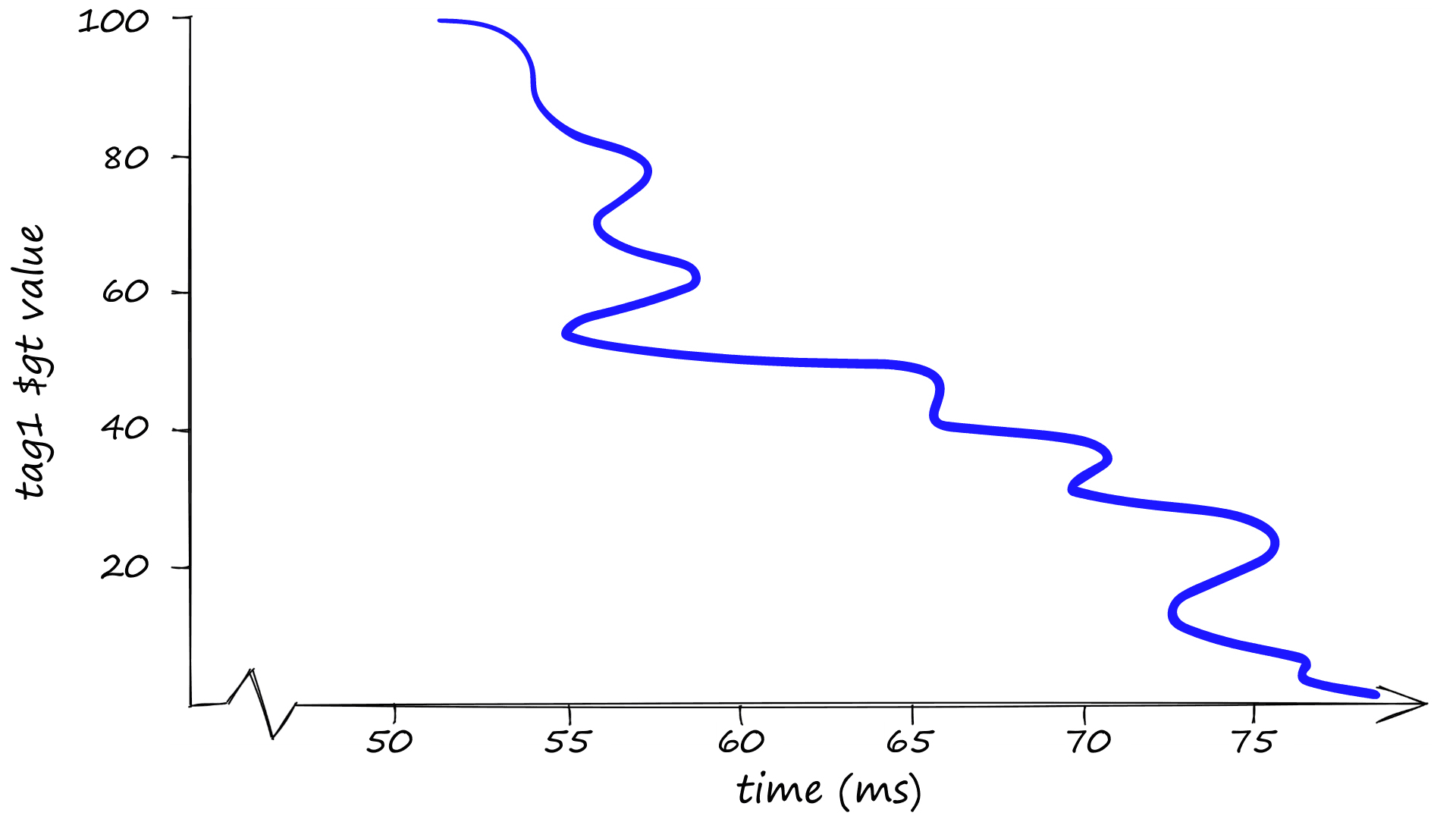
As we increase our tag1 $gt value, the search scope is reduced, making our search with the single-stage filter even faster.
And that’s it! We explored the flexible filter queries and tested the impressive search speeds of the single-stage filter!
Thanks for following with us through the three approaches to metadata filtering in vector similarity search; pre-filtering, post-filtering, and Pinecone’s single-stage filtering.
We hope the article has been helpful! Now you can try our single-stage filtering for your own vector search application.
此内容由惯性聚合(RSS阅读器)自动聚合整理,仅供阅读参考。 原文来自 — 版权归原作者所有。