








Evaluation of information retrieval (IR) systems is critical to making well-informed design decisions. From search to recommendations, evaluation measures are paramount to understanding what does and does not work in retrieval.
Many big tech companies contribute much of their success to well-built IR systems. One of Amazon’s earliest iterations of the technology was reportedly driving more than 35% of their sales[1]. Google attributes 70% of YouTube views to their IR recommender systems[2][3].
IR systems power some of the greatest companies in the world, and behind every successful IR system is a set of evaluation measures.
Evaluation measures for IR systems can be split into two categories: online or offline metrics.
Online metrics are captured during actual usage of the IR system when it is online. These consider user interactions like whether a user clicked on a recommended show from Netflix or if a particular link was clicked from an email advertisement (the click-through rate or CTR). There are many online metrics, but they all relate to some form of user interaction.
Offline metrics are measured in an isolated environment before deploying a new IR system. These look at whether a particular set of relevant results are returned when retrieving items with the system.
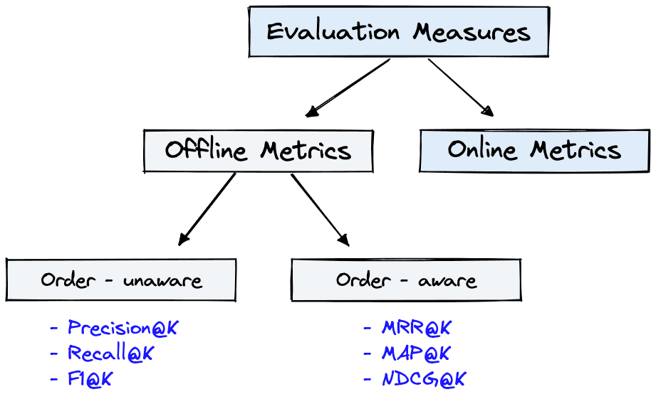
Evaluation measures can be categorized as either offline or online metrics. Offline metrics can be further divided into order-unaware or order-aware, which we will explain soon.
Organizations often use both offline and online metrics to measure the performance of their IR systems. It begins, however, with offline metrics to predict the system’s performance before deployment.
We will focus on the most useful and popular offline metrics:
These metrics are deceptively simple yet provide invaluable insight into the performance of IR systems.
We can use one or more of these metrics in different evaluation stages. During the development of Spotify’s podcast search; Recall@K (using ) was used during training on “evaluation batches”, and after training, both Recall@K and MRR (using ) were used with a much larger evaluation set.
The last paragraph will make sense by the end of this article. For now, understand that Spotify was able to predict system performance before deploying anything to customers. This allowed them to deploy successful A/B tests and significantly increase podcast engagement[4].
We have two more subdivisions for these metrics; order-aware and order-unaware. This refers to whether the order of results impacts the metric score. If so, the metric is order-aware. Otherwise, it is order-unaware.
Throughout the article, we will be using a very small dataset of eight images. In reality, this number is likely to be millions or more.

Example query and ranking of the eight possible results.
If we were to search for “cat in a box”, we may return something like the above. The numbers represent the relevance rank of each image as predicted by the IR system. Other queries would yield a different order of results.

Example query and ranking with actual relevant results highlighted.
We can see that results 2, 4, 5, and 7 are actual relevant results. The other results are not relevant as they show cats without boxes, boxes without cats, or a dog.
When evaluating the performance of the IR system, we will be comparing actual vs. predicted conditions, where:
From these actual and predicted conditions, we create a set of outputs from which we calculate all of our offline metrics. Those are the true/false positives and true/false negatives.
The positive results focus on what the IR system returns. Given our dataset, we ask the IR system to return two items using the “cat in a box” query. If it returns an actual relevant result this is a true positive (); if it returns an irrelevant result, we have a false positive ().
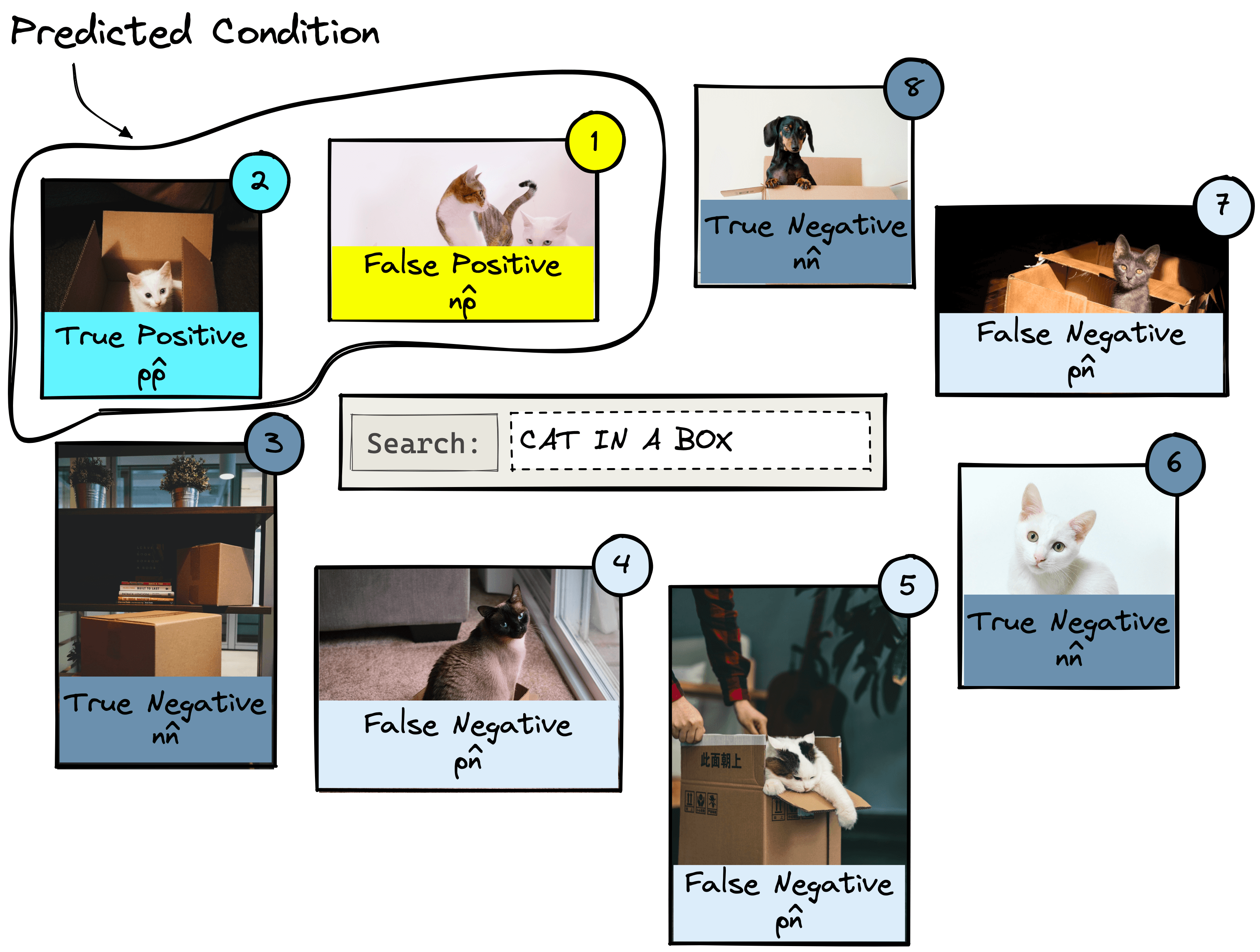
For negative results, we must look at what the IR system does not return. Let’s query for two results. Anything that is relevant but is not returned is a false negative (). Irrelevant items that were not returned are true negatives ().
With all of this in mind, we can begin with the first metric.
Recall@K is one of the most interpretable and popular offline evaluation metrics. It measures how many relevant items were returned () against how many relevant items exist in the entire dataset ().
The K in this and all other offline metrics refers to the number of items returned by the IR system. In our example, we have a total number of N = 8 items in the entire dataset, so K can be any value between .

With recall@2 we return the predicted top K = 2 most relevant results.
When K = 2, our recall@2 score is calculated as the number of returned relevant results over the total number of relevant results in the entire dataset. That is:
With recall@K, the score improves as K increases and the scope of returned items increases.
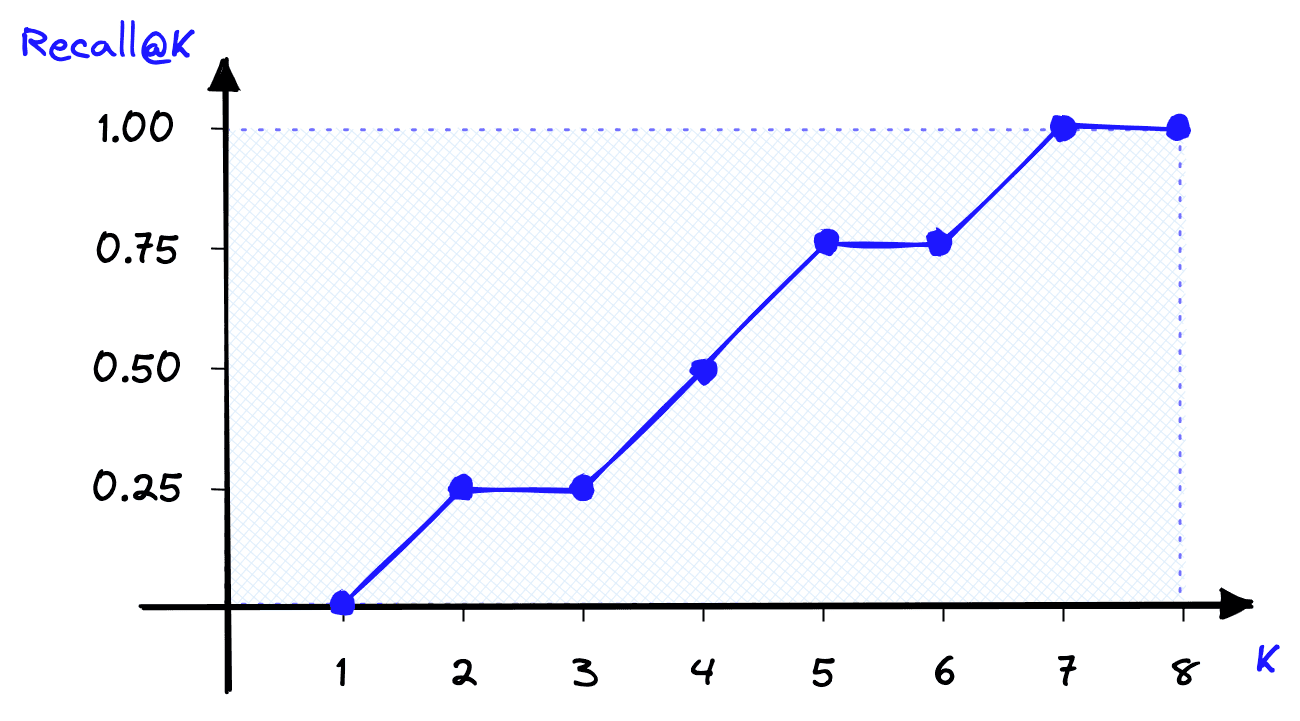
With recall@K we will see the score increase as K increases and more positives (whether true or false) are returned.
We can calculate the same recall@K score easily in Python. For this, we will define a function named recall that takes lists of actual conditions and predicted conditions, a K value, and returns a recall@K score.
# recall@k function
def recall(actual, predicted, k):
    act_set = set(actual)
    pred_set = set(predicted[:k])
    result = round(len(act_set & pred_set) / float(len(act_set)), 2)
    return result
Using this, we will replicate our eight-image dataset with actual relevant results in rank positions 2, 4, 5, and 7.
In[2]:
actual = ["2", "4", "5", "7"]
predicted = ["1", "2", "3", "4", "5", "6", "7", "8"]
for k in range(1, 9):
    print(f"Recall@{k} = {recall(actual, predicted, k)}")
Out[2]:
Recall@1 = 0.0
Recall@2 = 0.25
Recall@3 = 0.25
Recall@4 = 0.5
Recall@5 = 0.75
Recall@6 = 0.75
Recall@7 = 1.0
Recall@8 = 1.0
Recall@K is undoubtedly one of the most easily interpretable evaluation metrics. We know that a perfect score indicates that all relevant items are being returned. We also know that a smaller k value makes it harder for the IR system to score well with recall@K.
Still, there are disadvantages to using recall@K. By increasing K to N or near N, we can return a perfect score every time, so relying solely on recall@K can be deceptive.
Another problem is that it is an order-unaware metric. That means if we used recall@4 and returned one relevant result at rank one, we would score the same as if we returned the same result at rank four. Clearly, it is better to return the actual relevant result at a higher rank, but recall@K cannot account for this.
The Mean Reciprocal Rank (MRR) is an order-aware metric, which means that, unlike recall@K, returning an actual relevant result at rank one scores better than at rank four.
Another differentiator for MRR is that it is calculated based on multiple queries. It is calculated as:
is the number of queries, a specific query, and the rank of the first *actual relevant* result for query . We will explain the formula step-by-step.
Using our last example where a user searches for “cat in a box”. We add two more queries, giving us .
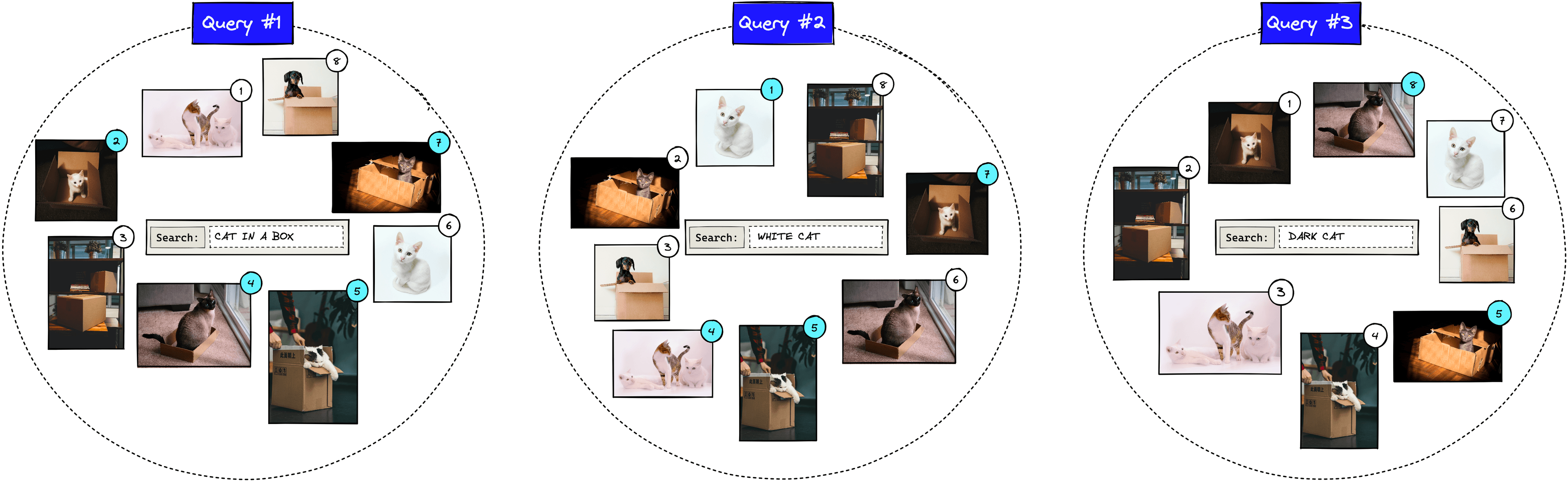
We perform three queries while calculating the MRR score.
We calculate the rank reciprocal for each query . For the first query, the first actual relevant image is returned at position two, so the rank reciprocal is . Let’s calculate the reciprocal rank for all queries:
Next, we sum all of these reciprocal ranks for queries (e.g., all three of our queries):
As we are calculating the mean reciprocal rank (MRR), we must take the average value by dividing our total reciprocal ranks by the number of queries :
Now let’s translate this into Python. We will replicate the same scenario where using the same actual relevant results.
In[1]:
# relevant results for query #1, #2, and #3
actual_relevant = [
    [2, 4, 5, 7],
    [1, 4, 5, 7],
    [5, 8]
]
In[2]:
# number of queries
Q = len(actual_relevant)

# calculate the reciprocal of the first actual relevant rank
cumulative_reciprocal = 0
for i in range(Q):
    first_result = actual_relevant[i][0]
    reciprocal = 1 / first_result
    cumulative_reciprocal += reciprocal
    print(f"query #{i+1} = 1/{first_result} = {reciprocal}")

# calculate mrr
mrr = 1/Q * cumulative_reciprocal

# generate results
print("MRR =", round(mrr,2))
Out[2]:
query #1 = 1/2 = 0.5
query #2 = 1/1 = 1.0
query #3 = 1/5 = 0.2
MRR = 0.57
And as expected, we calculate the same MRR score of 0.57.
MRR has its own unique set of advantages and disadvantages. It is order-aware, a massive advantage for use cases where the rank of the first relevant result is important, like chatbots or question-answering.
On the other hand, we consider the rank of the first relevant item, but no others. That means for use cases where we’d like to return multiple items like recommendation or search engines, MRR is not a good metric. For example, if we’d like to recommend ~10 products to a user, we ask the IR system to retrieve 10 items. We could return just one actual relevant item in rank one and no other relevant items. Nine of ten irrelevant items is a terrible result, but MRR would score a perfect 1.0.
Another minor disadvantage is that MRR is less readily interpretable compared to a simpler metric like recall@K. However, it is still more interpretable than many other evaluation metrics.
Mean Average Precision@K (MAP@K) is another popular order-aware metric. At first, it seems to have an odd name, a mean of an average? It makes sense; we promise.
There are a few steps to calculating MAP@K. We start with another metric called precision@K:
You may be think this looks very similar to recall@K, and it is! The only difference is that we’ve swapped in recall for here. That means we now consider both actual relevant and non-relevant results only from the returned items. We do not consider non-returned items with precision@K.
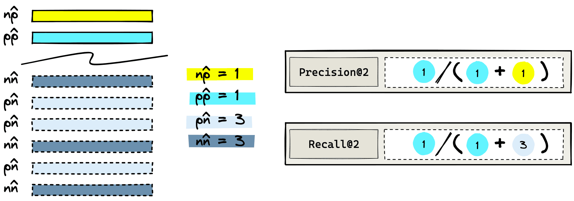
The difference between Recall@K and Precision@K calculation where K = 2.
Let’s return to the “cat in a box” example. We will return items and calculate precision@2.
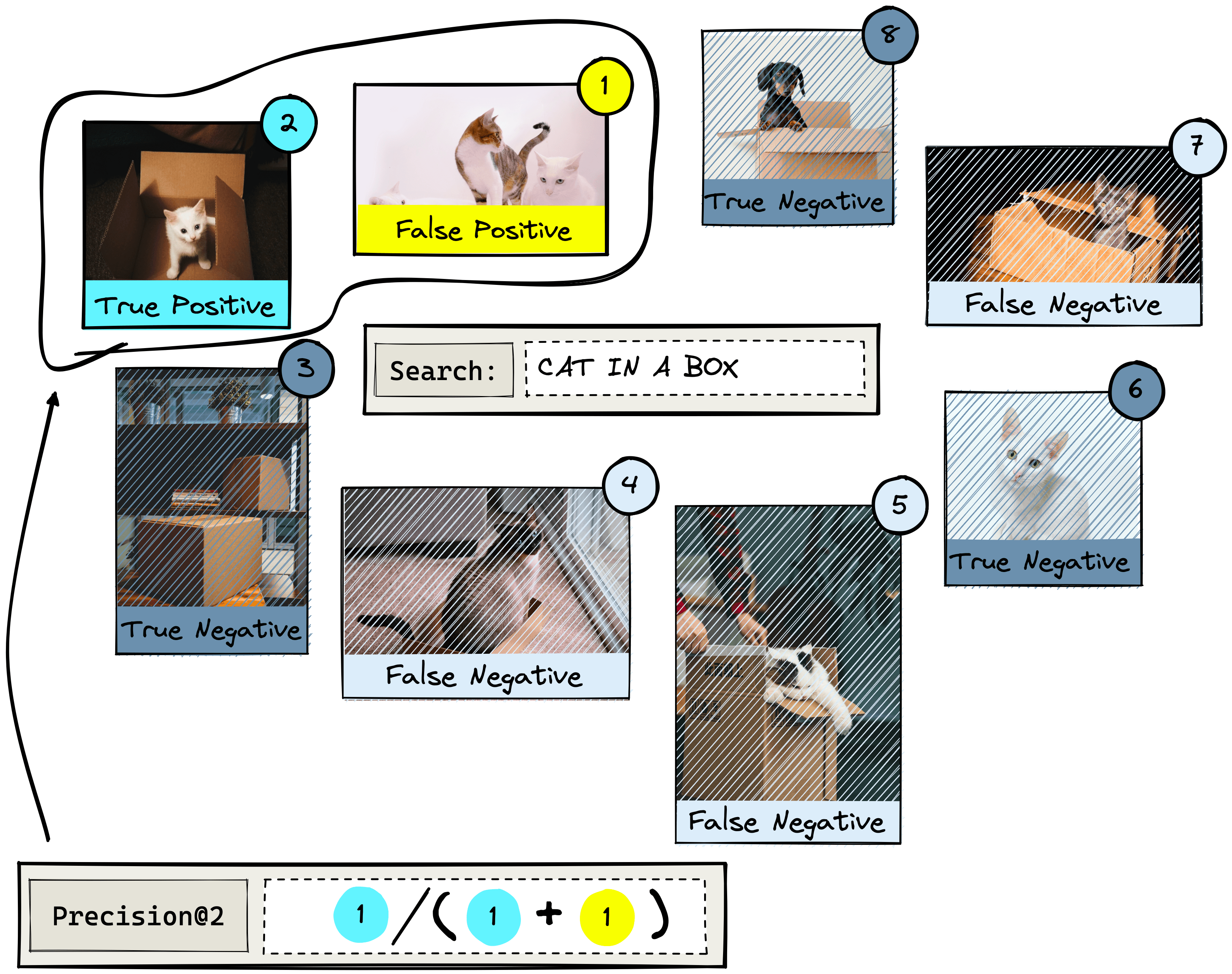
Precision@K calculation where K = 2.
Note that the denominator in precision@K always equals . Now that we have the precision@K value, we move on to the next step of calculating the Average Precision@K (AP@K):
Note that for AP@K we are taking the average precision@k score for all values of . Meaning that for AP@5 we calculate precision@k where .
We have not seen the parameter before. It is a relevance parameter that (for AP@K) is equal to 1 when the item is relevant or 0 when it is not.
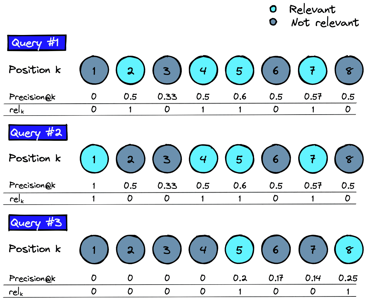
We calculate precision@k and iteratively using .
As we multiply precision@k and , we only need to consider precision@k where the item is relevant.
![Precision@k and rel_k values for all relevant items across three queries q = [1, ..., Q]](https://www.pinecone.io/_next/image/?url=https%3A%2F%2Fcdn.sanity.io%2Fimages%2Fvr8gru94%2Fproduction%2F5bbb920bf69343baedc4b93d2f7a48c576a18d77-737x1005.png&w=1920&q=75)
Precision@k and rel_k values for all relevant items across three queries q = [1, ..., Q]
Given these values, for each query , we can calculate the score where as:
Each of these individual calculations produces a single Average Precision@K score for each query q�. To get the Mean Average Precision@K (MAP@K) score for all queries, we simply divide by the number of queries :
That leaves us with a final MAP@K score of 0.48. To calculate all of this with Python, we write:
In[1]:
# initialize variables
actual = [
    [2, 4, 5, 7],
    [1, 4, 5, 7],
    [5, 8]
]
Q = len(actual)
predicted = [1, 2, 3, 4, 5, 6, 7, 8]
k = 8
ap = []

# loop through and calculate AP for each query q
for q in range(Q):
    ap_num = 0
    # loop through k values
    for x in range(k):
        # calculate precision@k
        act_set = set(actual[q])
        pred_set = set(predicted[:x+1])
        precision_at_k = len(act_set & pred_set) / (x+1)
        # calculate rel_k values
        if predicted[x] in actual[q]:
            rel_k = 1
        else:
            rel_k = 0
        # calculate numerator value for ap
        ap_num += precision_at_k * rel_k
    # now we calculate the AP value as the average of AP
    # numerator values
    ap_q = ap_num / len(actual[q])
    print(f"AP@{k}_{q+1} = {round(ap_q,2)}")
    ap.append(ap_q)

# now we take the mean of all ap values to get mAP
map_at_k = sum(ap) / Q

# generate results
print(f"mAP@{k} = {round(map_at_k, 2)}")
Out[1]:
AP@8_1 = 0.54
AP@8_2 = 0.67
AP@8_3 = 0.23
mAP@8 = 0.48
Returning the same MAP@K score of 0.480.48.
MAP@K is a simple offline metric that allows us to consider the order of returned items. Making this ideal for use cases where we expect to return multiple relevant items.
The primary disadvantage of MAP@K is the relevance parameter is binary. We must either view items as relevant or irrelevant. It does not allow for items to be slightly more/less relevant than others.
Normalized Discounted Cumulative Gain @K () is another order-aware metric that we can derive from a few simpler metrics. Starting with Cumulative Gain () calculated like so:
The variable is different this time. It is a range of relevance ranks where *0* is the least relevant, and some higher value is the most relevant. The number of ranks does not matter; in our example, we use a range of .
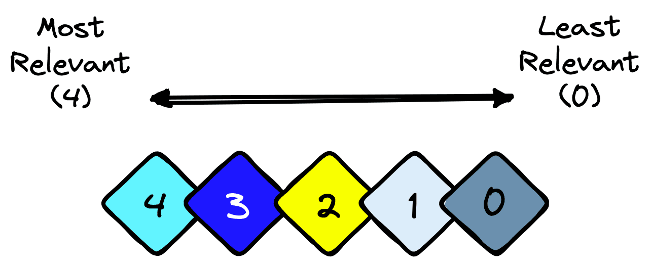
Using rel_k we rank every item based on its relevance to a particular query q.
Let’s try applying this to another example. We will use a similar eight-image dataset as before. The circled numbers represent the IR system’s predicted ranking, and the diamond shapes represent the actual ranking.
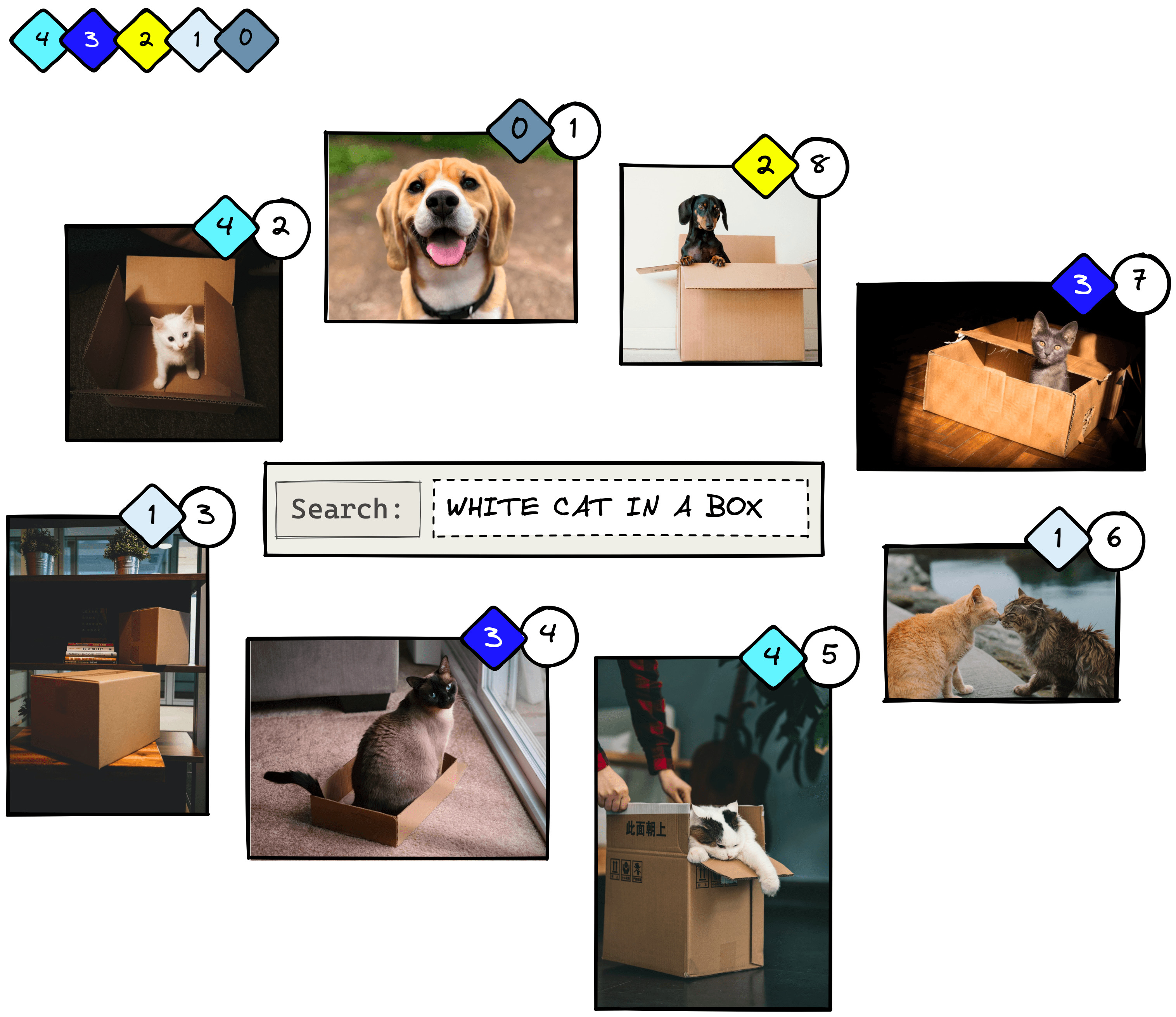
A small dataset with predicted ranks (circles) and actual ranks (diamonds).
To calculate the cumulative gain at position K (CG@K), we sum the relevance scores up to the predicted rank K. When :
It’s important to note that CG@K is not order-aware. If we swap images 1 and 2, we will return the same score when despite having the more relevant item placed first.

Images 1 and 2 have been swapped.
To handle this lack of order awareness, we modify the metric to create DCG@K, adding a penalty in the form of to the formula:
Now when we calculate DCG@2 and swap the position of the first two images, we return different scores:
from math import log2

# initialize variables
relevance = [0, 7, 2, 4, 6, 1, 4, 3]
K = 8

dcg = 0
# loop through each item and calculate DCG
for k in range(1, K+1):
    rel_k = relevance[k-1]
    # calculate DCG
    dcg += rel_k / log2(1 + k)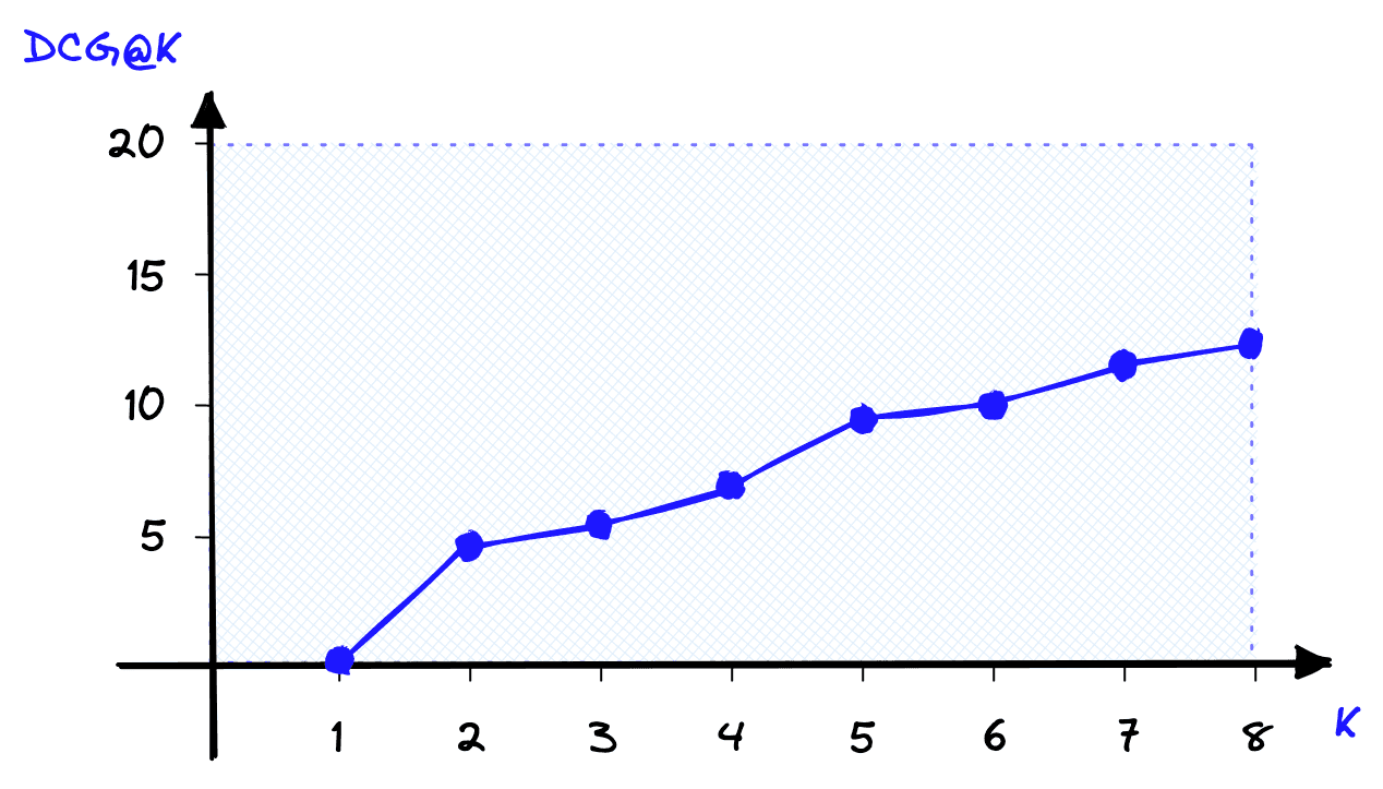
DCG@K score as K increases using the query #1 order of results.
Using the order-aware metric means the preferred swapped results returns a better score.
Unfortunately, DCG@K scores are very hard to interpret as their range depends on the variable range we chose for our data. We use the Normalized DCG@K (NDCG@K) metric to fix this.
NDCG@K is a special modification of standard NDCG that cuts off any results whose rank is greater than K. This modification is prevalent in use-cases measuring search performance[5].
NDCG@K normalizes DCG@K using the Ideal DCG@K (IDCG@K) rankings. For IDCG@K, we assume that the most relevant items are ranked highest and in order of relevance.
Calculating IDCG@K takes nothing more than reordering the assigned ranks and performing the same DCG@K calculation:
# sort items in 'relevance' from most relevant to less relevant
ideal_relevance = sorted(relevance, reverse=True)

print(ideal_relevance)

idcg = 0
# as before, loop through each item and calculate *Ideal* DCG
for k in range(1, K+1):
    rel_k = ideal_relevance[k-1]
    # calculate DCG
    idcg += rel_k / log2(1 + k)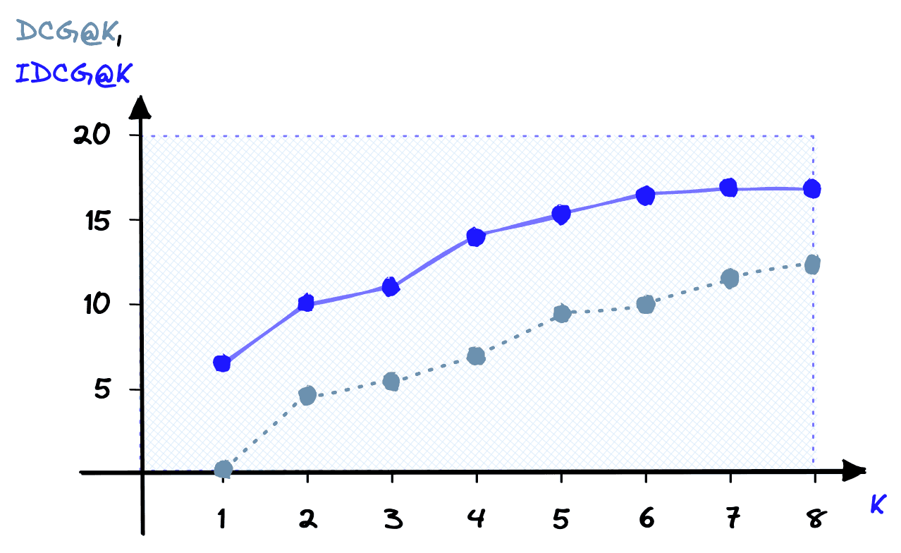
IDCG@K score as K increases compared against the DCG@K score calculated with using the query #1 order of results.
Now all we need to calculate NDCG@K is to normalize our DCG@K score using the IDCG@K score:
dcg = 0
idcg = 0

for k in range(1, K+1):
    # calculate rel_k values
    rel_k = relevance[k-1]
    ideal_rel_k = ideal_relevance[k-1]
    # calculate dcg and idcg
    dcg += rel_k / log2(1 + k)
    idcg += ideal_rel_k / log2(1 + k)
    # calcualte ndcg
    ndcg = dcg / idcg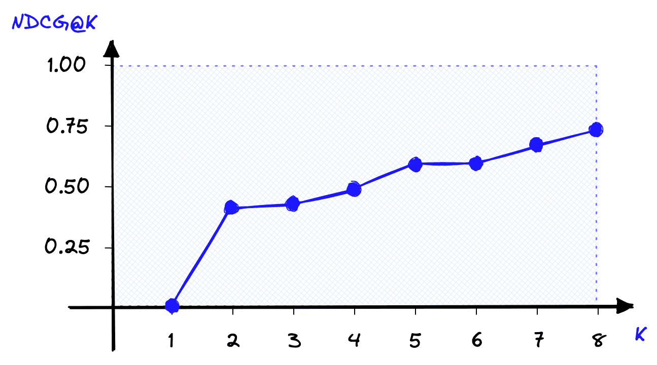
NDCG@K score as K increases calculated by normalizing DCG@K using IDCG@K.
Using NDCG@K, we get a more interpretable result of 0.41, where we know that 1.0 is the best score we can get with all items ranked perfectly (e.g., the IDCG@K).
NDCG@K is one of the most popular offline metrics for evaluating IR systems, in particular web search engines. That is because NDCG@K optimizes for highly relevant documents, is order-aware, and is easily interpretable.
However, there is a significant disadvantage to NDCG@K. Not only do we need to know which items are relevant for a particular query, but we need to know whether each item is more/less relevant than other items; the data requirements are more complex.
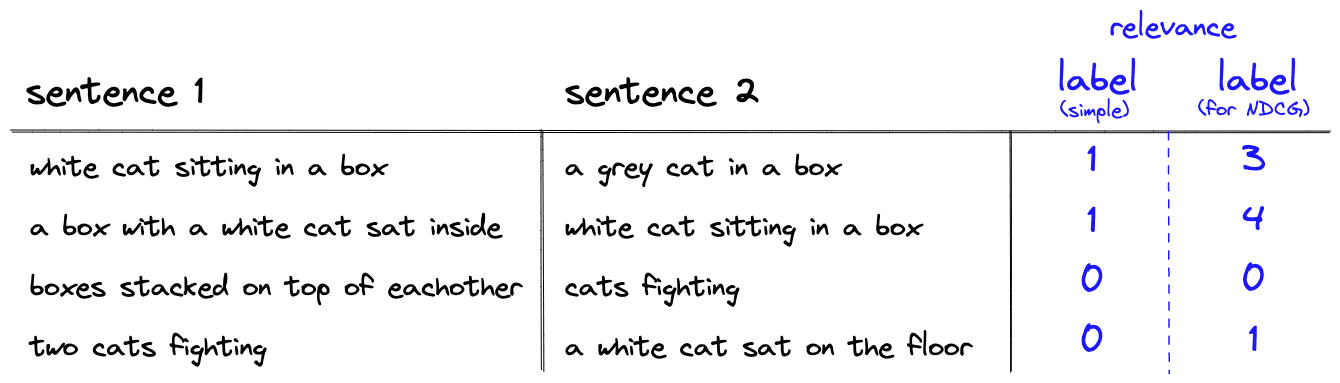
Example of data for the other metrics (left) and the more complex data required for NDCG@K (right).
These are some of the most popular offline metrics for evaluating information retrieval systems. A single metric can be a good indicator of system performance. For even more confidence in retrieval performance you can use several metrics, just as Spotify did with recall@1, recall@30, and MRR@30.
These metrics are still best supported with online metrics during A/B testing, which act as the next step before deploying your retrieval system to the world. However, these offline metrics are the foundation behind any retrieval project.
Whether you’re prototyping your very first product, or evaluating the latest iteration of Google search, evaluating your retrieval system with these metrics will help you deploy the best retrieval system possible.
[1] G. Linden et al., Item-to-Item Collaborative Filtering (2003), IEEE
[2] J. Solsman, YouTube’s AI is the puppet master over most of what you watch (2018)
[3] P. Covington et al., Deep Neural Networks for YouTube Recommendations (2016), RecSys
[4] A. Tamborrino, Introducing Natural Language Search for Podcast Episodes (2022), Engineering at Spotify Blog
[5] Y. Wang et al., A Theoretical Analysis of NDCG Ranking Measures (2013), JMLR
此内容由惯性聚合(RSS阅读器)自动聚合整理,仅供阅读参考。 原文来自 — 版权归原作者所有。