


Open-domain question-answering (ODQA) is a wildly popular pipeline of databases and language models that allow us to ask a machine human-like questions and return comprehensible and even intelligent answers.
Despite the outward guise of simplicity, ODQA requires a reasonably advanced set of components placed together to enable the extractive Q&A functionality.
We call this extractive Q&A because the models are not generating an answer. Instead, the answer already exists but is hidden somewhere within potentially thousands, millions, or even more data sources.
By enabling extractive Q&A, we enable a more intelligent and efficient way to retrieve information from what can be massive stores of data.
ODQA relies on three components: the vector database, for storing encoded vector representations of the data we will search, a retriever to handle context and question encoding, and a reader model that consumes relevant retrieved contexts and identifies a shorter, more specific answer.
The reader is the final act in an ODQA pipeline; it takes the contexts returned by the vector database and retriever components and reads them. Our reader will then return what it believes to be the specific answer to our question.
To be exact, we don’t get the ‘specific answer’. The model is reading input IDs, which are integers representing words or subwords. So, rather than returning a human-readable text answer, it actually returns a span of input ID positions.
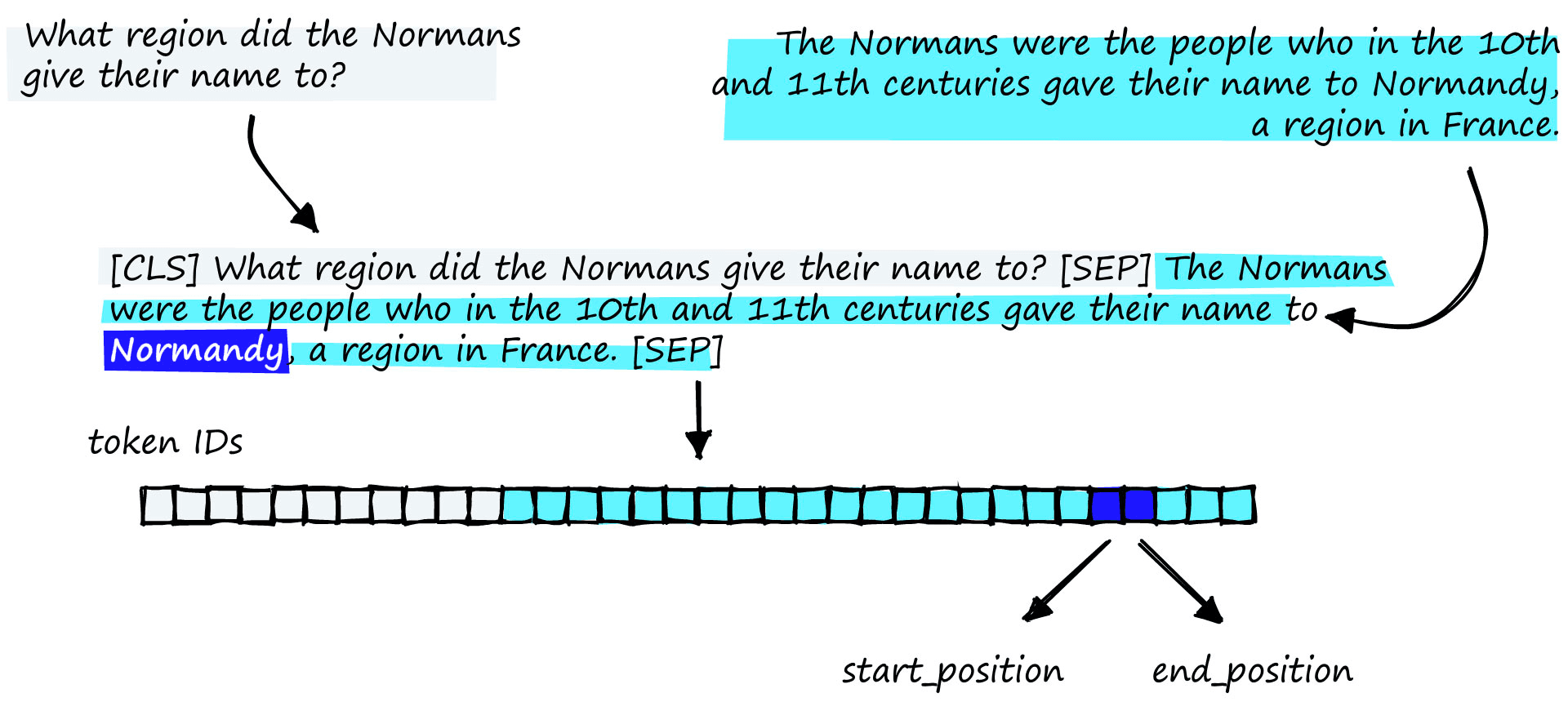
Question (grey), context (cyan), and answer (blue). The model doesn’t read the strings. It reads token IDs, and so when outputting a prediction for the answer, it outputs a span of token IDs that it believes represent the answer.
To fine-tune a model, we need two inputs and two labels. The inputs are the question and a relevant context, and the labels are the answer’s start and end positions.
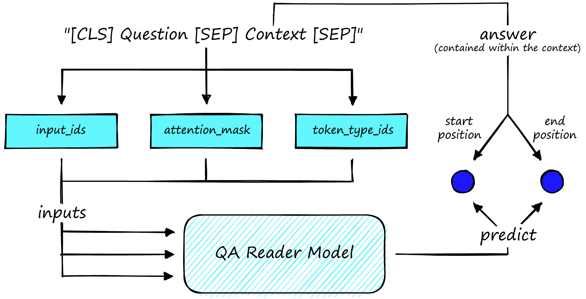
Inputs (cyan) and target labels (answer start and end positions, blue). The start and end positions are the token positions from the encoded question-context input_ids tensor that represent the start and end of the answer (extracted from the context).
There isn’t much more to fine-tuning a reader model. It’s a relatively straightforward process. The most complex part is pre-processing the training data.
With our overview complete, let’s dive into the details and work through an actual training example.
Implementation
There are more steps when training a reader model than just train the model. As mentioned, these other steps can prove to be the tricky part. In our case, we have three distinct steps.
- Download and pre-process Q&A dataset
- Fine-tune the model
- Evaluation
Without any further ado, let’s begin with the data.
Download and Pre-process
We will be using the Stanford Question and Answering Dataset (SQuAD) for fine-tuning. We can download it with HuggingFace Datasets.
In[1]:
from datasets import load_dataset

squad = load_dataset('squad_v2', split='train')
squad
Out[1]:
Dataset({
    features: ['id', 'title', 'context', 'question', 'answers'],
    num_rows: 130319
})
Looking at this, we have five features, of which we only care about question, context for the inputs, and answers for the labels.
Out[2]:
{'id': '56be85543aeaaa14008c9063',
 'title': 'Beyoncé',
 'context': 'Beyoncé Giselle Knowles-Carter (/biːˈjɒnseɪ/ bee-YON-say) (born September 4, 1981) is an American singer, songwriter, record producer and actress. Born and raised in Houston, Texas, she performed in various singing and dancing competitions as a child, and rose to fame in the late 1990s as lead singer...',
 'question': 'When did Beyonce start becoming popular?',
 'answers': {'answer_start': 269,
  'text': 'in the late 1990s'}}
We must make a few transformations to format the answers into the start and end token ID positions we need. We have answer_start, but this gives us the position within the context string that the answer begins. These positions are not what the model needs. Instead, it requires the start position using token ID indexes.
In[2]:
# we can get the end position of the answer
squad[0]['answers']['answer_start'][0] + len(squad[0]['answers']['text'][0])
In[3]:
squad[0]['context'][269:286]
# this works, but only for strings, not for the token IDs that we need for BERT
That is our main hurdle. To push through it, we will take three steps:
- Tokenize the context.
- Convert
answer_startto a token ID index. - Find the end token index using the starting position and answer
text.
Starting with tokenize the context, we first initialize a tokenizer using the HuggingFace Transformers library.
In[7]:
from transformers import BertTokenizerFast
# initialize the tokenizer
tokenizer = BertTokenizerFast.from_pretrained('bert-base-uncased')
In[8]:
# tokenize our question-context pairs
squad = squad.map(lambda x: tokenizer(
    x['question'], x['context'], max_length=384,
    padding='max_length', truncation=True,
    return_offsets_mapping=True
))
Then we tokenize our question-context pairs, and this returns three tensors by default:
input_ids, the token ID representation of our text.attention_maska list of values telling our model whether to apply the attention mechanism to respective token embeddings with1or to ignore padding token positions with0.token_type_idsindicates sentence A (the question) with the first set of0values, sentence B (the context) with1values, and remaining padding tokens with the trailing0values.
We have added another tensor called offset_mapping by setting return_offsets_mapping=True. This tensor is very important for finding our label values for training our model.
Earlier, we found the start and end positions for the character positions from our context string. As mentioned, we cannot use these. We need the token positions, and the offset_mapping tensor is essential in finding the token positions.
In[10]:
tokenizer.decode(squad[0]['input_ids'])Out[10]:
'[CLS] when did beyonce start becoming popular? [SEP] beyonce giselle knowles - carter ( / biːˈjɒnseɪ / bee - yon - say ) ( born september 4, 1981 ) is an american singer... singles " crazy in love " and " baby boy ". [SEP] [PAD] [PAD] [PAD] [PAD]...'Another consideration when finding the token position is that when we tokenized, we tokenized both the question and context as shown above where we follow the format [CLS] question [SEP] context [SEP] padding. To find the answer start and end positions, we must shift the values by the length of the question segment.
To find the question and context segment lengths, we use the token_type_ids tensor.
In[12]:
question_len = 0
# get question length by identifying where 0 tokens first stop
for x in squad[0]['token_type_ids']:
    if x != 1:
        question_len += 1
    else: break
# context is represented by 1s, so we take a sum to get context len
context_len = sum(squad[0]['token_type_ids'])
question_len, context_len
We need to consider one additional case where the answer has been truncated or never existed (some records have no answer). In both of these scenarios, we set the start and end positions to 0.
In[34]:
def char_to_id(sample):
    char_start = sample['answers']['answer_start']
    char_end = sample['answers']['answer_end']
    # find the question length
    question_len = 0
    for x in sample['token_type_ids']:
        if x != 1:
            question_len += 1
        else: break
    # and get the context length
    context_len = sum(sample['token_type_ids'])
    # get offset mappings for context segment
    context_mappings = sample['offset_mapping'][question_len:][:context_len-1]
    for i, mapping in enumerate(context_mappings):
        if char_start >= mapping[0] and char_start <= mapping[1]:
            token_start = question_len + i
        if char_end >= mapping[0] and char_end <= mapping[1]:
            token_end = question_len + i + 1
            return {'start_positions': token_start, 'end_positions': token_end}
        if i == len(context_mappings) - 1:
            # this means the answer tokens are out of range, eg have been truncated
            # and therefore there is no answer
            token_start, token_end = 0, 0
            return {'start_positions': token_start, 'end_positions': token_end}
In[36]:
squad = squad.map(lambda x: char_to_id(x))Out[36]:
100%|██████████| 130319/130319 [02:56<00:00, 737.32ex/s]
Out[37]:
{'id': '56be85543aeaaa14008c9063',
 'title': 'Beyoncé',
 'context': 'Beyoncé Giselle Knowles-Carter... singles "Crazy in Love" and "Baby Boy".',
 'question': 'When did Beyonce start becoming popular?',
 'answers': {'answer_end': 286,
  'answer_start': 269,
  'text': 'in the late 1990s'},
 'input_ids': [...],
 'token_type_ids': [...],
 'attention_mask': [...],
 'offset_mapping': [...],
 'start_positions': 75,
 'end_positions': 79}
Once we have the start and end positions, we need to define how we will load the dataset into our model for training. At the moment, our dataset will return lists of dictionaries for each training batch.
We cannot feed lists of dictionaries into our model. Instead, we need to pull these dictionaries into single batch-size tensors. For that, we use the default_data_collator function.
In[39]:
# remove all unecessary columns (only need input_ids, attention_mask,
# token_type_ids, start_positions, end_positions)
squad = squad.remove_columns(['id', 'title', 'context', 'question', 'answers', 'offset_mapping'])
squad
Out[39]:
Dataset({
    features: ['input_ids', 'token_type_ids', 'attention_mask', 'start_positions', 'end_positions'],
    num_rows: 130319
})
In[42]:
from transformers import default_data_collator
# prepare format of data being fed into model
data_collator = default_data_collator
We don’t need to do anything else with our dataset or data collator for now, so we move on to the next step of fine-tuning.
Fine-tuning the Model
As mentioned, we will be fine-tuning the model using the HuggingFace Transformers Trainer class. To use this, we first need a model to fine-tune, which we load as usual with transformers.
In[40]:
from transformers import BertForQuestionAnswering

model = BertForQuestionAnswering.from_pretrained('bert-base-uncased')
Next, we set up the Trainer training parameters.
In[41]:
from transformers import TrainingArguments

batch_size = 24
epochs = 3

args = TrainingArguments(
    'bert-base-uncased-squad2',
    learning_rate=2e-5,
    per_device_train_batch_size=batch_size,
    num_train_epochs=epochs,
    weight_decay=0.1,
    warmup_steps=int(len(squad)*epochs*0.1)
)
We use tried and testing training parameters used in the first BERT for QA with SQuADv2 paper and Deepset AI’s BERT training parameters, we set a learning rate of 2e-5, 0.1 weight decay, and train in batches of 24 for 3 epochs [1] [2].
In[43]:
from transformers import Trainer
import torch

device = 'cuda:0' if torch.cuda.is_available() else 'cpu'

trainer = Trainer(
    model.to(device),
    args,
    train_dataset=squad,
    data_collator=data_collator,
    tokenizer=tokenizer
)
Out[44]:
***** Running training *****
  Num examples = 130319
  Num Epochs = 3
  Instantaneous batch size per device = 24
  Total train batch size (w. parallel, distributed & accumulation) = 24
  Gradient Accumulation steps = 1
  Total optimization steps = 16290
  3%|▎         | 500/16290 [02:45<1:27:11,  3.02it/s]Saving model checkpoint to bert-base-uncased-squad2...
Out[44]:
Model weights saved in bert-base-uncased-squad2\checkpoint-16000\pytorch_model.bin
tokenizer config file saved in bert-base-uncased-squad2\checkpoint-16000\tokenizer_config.json
Special tokens file saved in bert-base-uncased-squad2\checkpoint-16000\special_tokens_map.json
100%|██████████| 16290/16290 [1:26:22<00:00,  3.24it/s]

Training completed. Do not forget to share your model on huggingface.co/models =)


100%|██████████| 16290/16290 [1:26:22<00:00,  3.14it/s]
Out[44]:
{'train_runtime': 5182.0739, 'train_samples_per_second': 75.444, 'train_steps_per_second': 3.144, 'train_loss': 2.052677161566241, 'epoch': 3.0}
Out[44]:
TrainOutput(global_step=16290, training_loss=2.052677161566241, metrics={'train_runtime': 5182.0739, 'train_samples_per_second': 75.444, 'train_steps_per_second': 3.144, 'train_loss': 2.052677161566241, 'epoch': 3.0})Like we said, fine-tuning the model is the easy part. We can find our model files in the directory defined in the args parameter, in this case, ./bert-base-uncased-squad2. We will see a set of folders named checkpoint-x in this directory. The last of those is the latest model checkpoint saved during training.
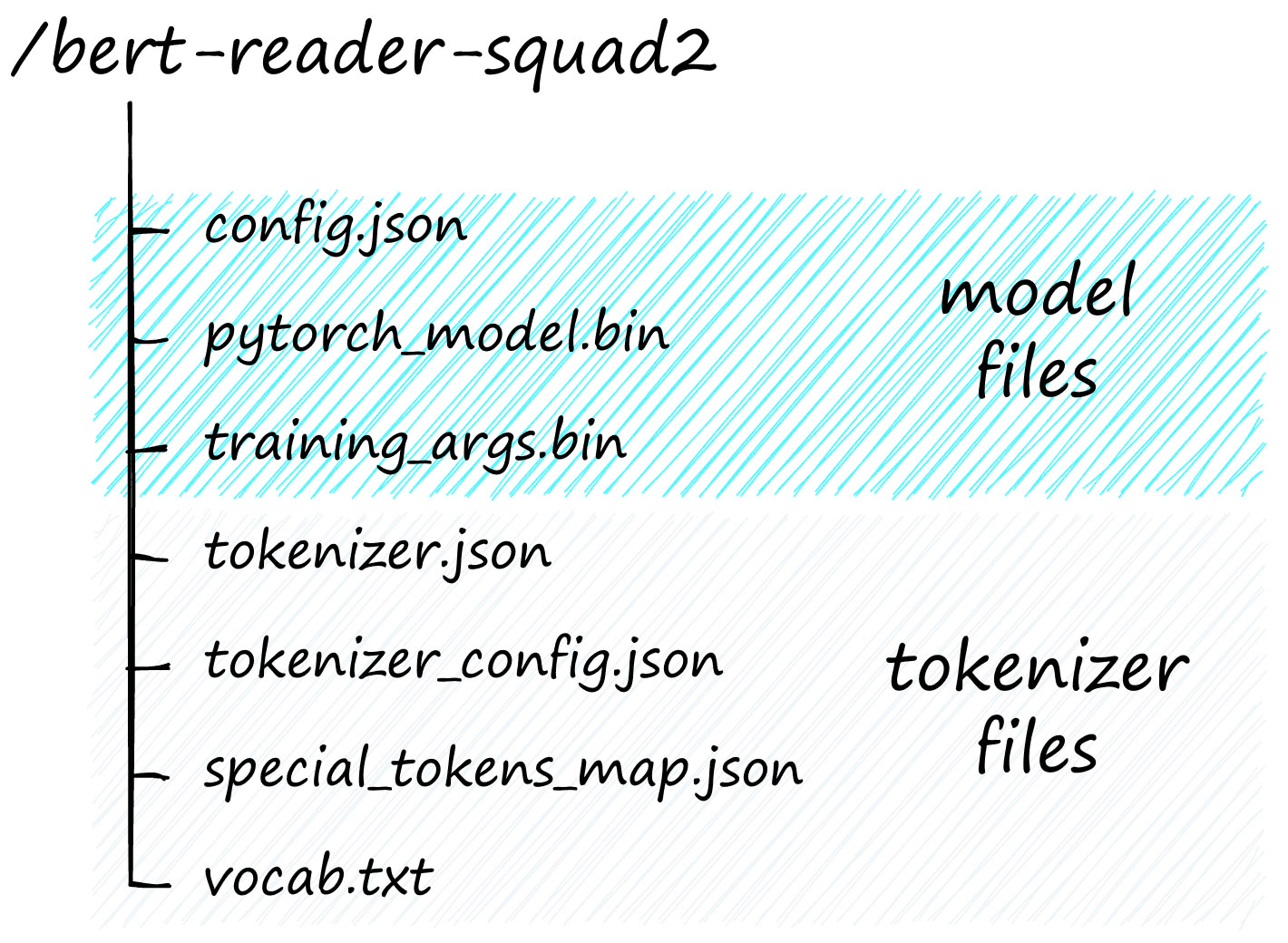
Model and tokenizer files in the /bert-reader-squad2 model directory.
By default, a new checkpoint is saved every 500 steps. These checkpoint saves mean the final model (at step 27,150) is not the final model but rather the model at step 27,000.
There is unlikely to be a noticeable difference between these two states, so we either take the model files from ./bert-base-uncased-squad2/checkpoint-24000 or we manually save our model with:
In[45]:
trainer.save_model('bert-reader-squad2')Out[45]:
Saving model checkpoint to bert-reader-squad2
Configuration saved in bert-reader-squad2\config.json
Model weights saved in bert-reader-squad2\pytorch_model.bin
tokenizer config file saved in bert-reader-squad2\tokenizer_config.json
Special tokens file saved in bert-reader-squad2\special_tokens_map.json
We can find the model files in the specified directory.
Inference
Before moving on to the next step of evaluation, let’s take a look at how we can use this model.
First, we initialize a transformers pipeline.
In[33]:
from transformers import pipeline

model_name = 'bert-reader-squad2'

qa = pipeline(
    'question-answering',
    model=model_name,
    tokenizer=model_name
)
Next, we prepare the evaluation data. Again we will use the squad_v2 dataset from HuggingFace, taking the validation split.
In[34]:
from datasets import load_dataset

dev = load_dataset('squad_v2', split='validation')
dev
Out[34]:
Dataset({
    features: ['id', 'title', 'context', 'question', 'answers'],
    num_rows: 11873
})
The pipeline requires an iterable set of key-value pairs where the only keys are question and context. We can simply drop the unneeded columns of id and title to handle this. However, we will need to keep track of the true answers during the next step of evaluation, so we store them in a separate ans dataset.
In[7]:
ans = dev['answers']
dev = dev.remove_columns(['id', 'title', 'answers'])
To make a prediction, we take a single question and context and feed them into our pipeline qa:
In[6]:
qa({
    'question': dev[1]['question'],
    'context': context
})
Out[6]:
{'score': 0.7120676040649414,
 'start': 94,
 'end': 122,
 'answer': '10th and 11th centuries gave'}
We’ll process the whole dataset like this in the next section.
Evaluation
We’ve technically finished fine-tuning our model, but it’s not of much use if we can’t validate its performance. We need confidence in the model’s performance.
Evaluation of our reader model is a little tricky as we want to identify matches between true and predicted answer labels. The most straightforward approach is to use an Exact Match metric. This metric will simply tell us 1 if the true and predicted answers are precisely the same or 0 if not.
There are two reasons we might want to avoid this and try something more flexible. First, we may find that a model predicts the correct answer, but when decoded, the predicted tokens are in a slightly different format.
The second reason is that our model might predict a partially correct answer and partially correct is better than nothing, but this better than nothing isn’t accounted for by the EM metric.
In[2]:
a = "the Normans"
b = "Normans"

exact_match = int(a == b)
rouge_score = rouge.get_scores(a, b)
exact_match, rouge_score
Out[2]:
(0,
 [{'rouge-1': {'r': 1.0, 'p': 0.5, 'f': 0.6666666622222223},
   'rouge-2': {'r': 0.0, 'p': 0.0, 'f': 0.0},
   'rouge-l': {'r': 1.0, 'p': 0.5, 'f': 0.6666666622222223}}])
We can solve the first issue in most cases by normalizing both the true and predicted answers, meaning we lowercase, remove punctuation, and remove any other potential points of conflict.
The second problem requires a more sophisticated solution, and it is best if we do not use the EM metric. Instead, we use ROUGE.
There are a few different ROUGE metrics. We will focus on ROUGE-N, which measures the number of matching n-grams between the predicted and true answers, where an n-gram is a grouping of tokens/words.
The N in ROUGE-N stands for the number of tokens/words within a single n-gram. This means that ROUGE-1 compares individual tokens/words (unigrams), ROUGE-2 compares tokens/words in chunks of two (bigrams), and so on.
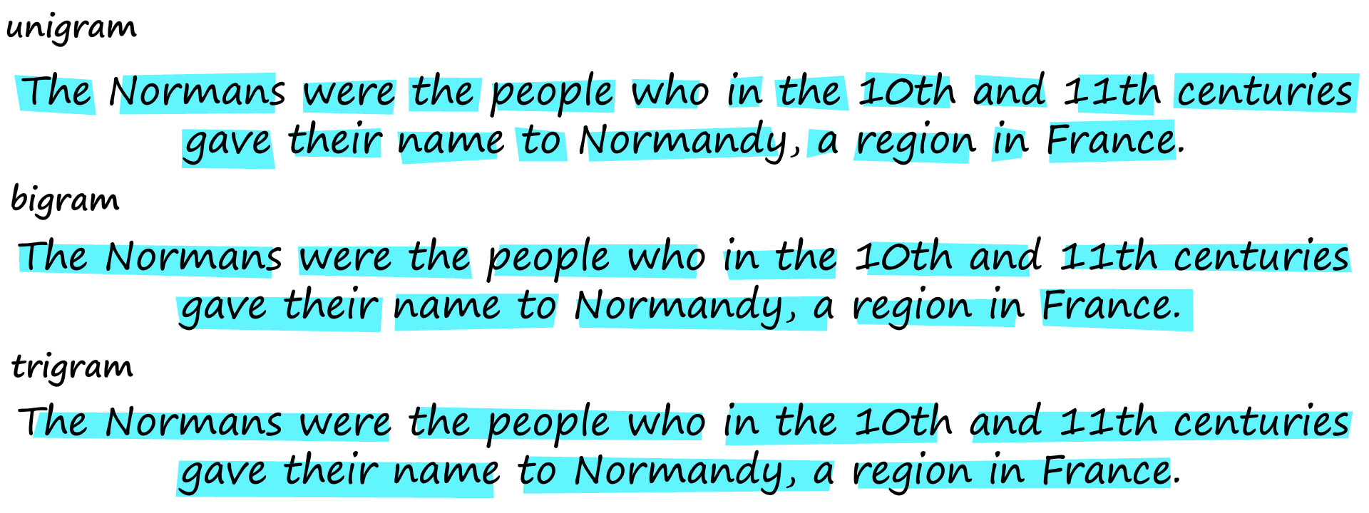
Example of unigram, bigram, and trigram which are single-token, double-token, and triple-token groupings respectively.
Either way, we return a score of 1 for an exact match, 0 for no match, or any value in between.
In[11]:
from rouge import Rouge

rouge = Rouge()
In[12]:
rouge.get_scores('hello this is an exact match', 'hello this is an exact match')Out[12]:
[{'rouge-1': {'r': 1.0, 'p': 1.0, 'f': 0.999999995},
  'rouge-2': {'r': 1.0, 'p': 1.0, 'f': 0.999999995},
  'rouge-l': {'r': 1.0, 'p': 1.0, 'f': 0.999999995}}]
In[13]:
rouge.get_scores('hello this is not a match', 'because nothing matches')Out[13]:
[{'rouge-1': {'r': 0.0, 'p': 0.0, 'f': 0.0},
  'rouge-2': {'r': 0.0, 'p': 0.0, 'f': 0.0},
  'rouge-l': {'r': 0.0, 'p': 0.0, 'f': 0.0}}]
In[14]:
rouge.get_scores('this is a half match', 'because half is matching')Out[14]:
[{'rouge-1': {'r': 0.5, 'p': 0.4, 'f': 0.4444444395061729},
  'rouge-2': {'r': 0.0, 'p': 0.0, 'f': 0.0},
  'rouge-l': {'r': 0.25, 'p': 0.2, 'f': 0.22222221728395072}}]
To apply ROUGE-1 for measuring reader model performance, we first need to predict answers using our model. We can then compare these predicted answers to the true answers.
In[8]:
results = []

for i in tqdm(range(len(dev))):
    out = qa(dev[i])
    results.append({
        **out,
        'true_answer': ans[i]['text']
    })
Out[8]:
100%|██████████| 11873/11873 [18:40<00:00, 10.59it/s]
Finally, given the two sets of answers, we can call rouge.get_scores to return recall r, precision p, and F1 f scores for both uni and bi-grams.
We still need to deal with where there is no answer and that the SQuAD evaluation set contains four possible answers for each sample.
Out[5]:
{'id': '56ddde6b9a695914005b9629',
 'title': 'Normans',
 'context': 'The Normans were the people who in the 10th and 11th centuries gave their name to Normandy, a region... over the succeeding centuries.',
 'question': 'When were the Normans in Normandy?',
 'answers': {'text': ['10th and 11th centuries',
   'in the 10th and 11th centuries',
   '10th and 11th centuries',
   '10th and 11th centuries'],
  'answer_start': [94, 87, 94, 94]}}
Out[10]:
{'id': '5ad39d53604f3c001a3fe8d1',
 'title': 'Normans',
 'context': 'The Normans were the people who in the 10th and 11th centuries gave their name to Normandy, a region... over the succeeding centuries.',
 'question': "Who gave their name to Normandy in the 1000's and 1100's",
 'answers': {'text': [], 'answer_start': []}}
We could check if the model correctly predicted that no answer exists for the ‘no answer’ scenario. If the model correctly identifies that there is no answer, we would return a score of 1.0. Otherwise, we would return a score of 0.0.
We will calculate the ROUGE-1 F1 score for every possible answer to deal with the multiple answers and take the best score.
After calculating all scores, we take the average value. This average value is the final ROUGE-1 F1 score for the model.
| Model | ROUGE-1 F1 |
|---|---|
| bert-reader-squad2 | 0.354 |
| deepset/bert-base-uncased-squad2 | 0.450 |
These scores seem surprisingly low. A big reason for this is the no answer scenarios. Let’s take a look at a few.
Out[20]:
{'context': 'The Normans were the people who in the 10th and 11th centuries gave their name to Normandy...',
 'question': "Who gave their name to Normandy in the 1000's and 1100's"}
Out[21]:
{'context': 'In the course of the 10th century, the initially destructive incursions of Norse war bands into the rivers of France evolved into more permanent encampments...',
 'question': 'when did Nors encampments ivolve into destructive incursions?'}
Out[22]:
{'context': '... Jerónimo de Ayanz y Beaumont received patents in 1606 for fifty steam powered inventions, including a water pump for draining inundated mines...',
 'question': 'In what year did Jeronimo de Ayanz y Beaumont patent a water pump for draining patients?'}
If, like me, you’re wondering how these are unanswerable, take note of the particular question and context wording. The first example specifies the 1000s and 1100s, but the context is the 10th and 11th centuries, e.g., 1100s and 1200s. The second example question should be "destructive incursions devolved into encampments". The third should be “draining mines".
Even by humans, each of these questions is easily mistaken as answerable. If we remove unanswerable examples, the model scores are less surprising.
| Model | ROUGE-1 F1 |
|---|---|
| bert-reader-squad2 | 0.708 |
| deepset/bert-base-uncased-squad2 | 0.901 |
The importance of identifying unanswerable questions varies between use cases. Many will not need to identify unanswerable questions, so question whether your models should prioritize unanswerable question identification or focus on performing well on answerable questions.
That’s it for this walkthrough in fine-tuning reader models for ODQA pipelines. By understanding how to fine-tune a QA reader model, we are able to effectively optimize the final step in the ODQA pipeline for our own specific use cases.
Pairing this with a custom vector database and retriever components allows us to add highly optimized ODQA capabilities to a variety of possible use cases, such as internal document search, e-commerce product discovery, or anything where a more natural information retrieval experience can be beneficial.
References
[1] Y. Zhang, Z. Xu, BERT for Question Answering on SQuAD 2.0 (2019)
[2] Model Card for deepset/bert-base-uncased-squad2, HuggingFace Model Hub
Was this article helpful?