





Google, Netflix, Amazon, and many more big tech companies all have one thing in common. They power their search and recommendation systems with “vector search”.
Before modern vector search, we had the “traditional” bag of words (BOW) methods. That is, we take a set of " documents" to be retrieved (like web pages on Google). Each document is transformed into a set (bag) of words, and use this to populate a sparse “frequency vector”. Popular algorithms for this include TF-IDF and BM25.
These sparse vectors are hugely popular in information retrieval thanks to their efficiency, interpretability, and exact term matching. Yet, they’re far from perfect.
Our nature as human beings does not align with sparse vector search. When searching for information, we rarely know the exact terms that will be contained in the documents we’re looking for.
Dense embedding models offer some help in this direction. By using dense models, we can search based on “semantic meaning” rather than term matching. However, these models could be better.
We need vast amounts of data to fine-tune dense embedding models; without this, they lack the performance of sparse methods. This is problematic for niche domains where data is hard to find and domain-specific terminology is important.
In the past, there have been a range of bandaid solutions for dealing with this; ranging from complex and (still not perfect) two-stage retrieval systems, to query and document expansion or rewrite methods (as we will explore later). However, none of these came close to being truly robust solutions.
Fortunately, plenty of progress has been made in making the most of both worlds. A merger of sparse and dense retrieval is now possible through hybrid search, and learnable sparse embeddings help minimize the traditional drawbacks of sparse retrieval.
This article will cover the latest in learnable sparse embeddings with SPLADE — the Sparse Lexical and Expansion model [1].
In information retrieval, vector embeddings represent documents and queries in a numerical vector format. This format allows us to search a vector database and identify similar vectors.
Sparse and dense vectors are two different forms of this representation, each with pros and cons.

Sparse vectors consist of many zero values with very few non-zero values.
Sparse vectors like TF-IDF or BM25 have high dimensionality and contain very few non-zero values (hence, they are called “sparse”). There are decades of research behind sparse vectors. Resulting in compact data structures and many efficient retireval algorithms designed specifically for these vectors.
Dense vectors are lower-dimensional but information-rich, with non-zero values in most-or-all dimensions. These are typically built using neural network models like transformers and, through this, can represent more abstract information like the semantic meaning behind some text.
Generally speaking, the pros and cons of both methods can be outlined as follows:
Sparse
| Pros | Cons |
|---|---|
| + Typically faster retrieval |
|
| + Good baseline performance |
|
| + Don’t need model fine-tuning |
|
| + Exact matching of terms |
Dense
| Pros | Cons |
|---|---|
| + Can outperform sparse with fine-tuning |
|
| + Search with human-like abstract concepts |
|
| + Multi-modality (text, images, audio, etc.) and cross-modal search (e.g., text-to-image) |
|
| |
|
Ideally, we want the merge the best of both, but that’s hard to do.
A typical approach to handling this is implementing a two-stage retrieval and ranking system. In this scenario, we use two distinct stages to retrieve and rank relevant documents for a given query.
In the first stage, the system uses a sparse retrieval method to retrieve a large set of candidate documents. These are then passed to the second stage, where we use a dense model to rerank the results based on their relevance to the query.
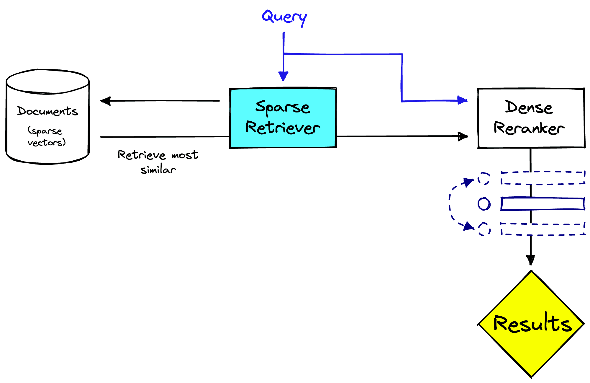
Two-stage retrieval system with a sparse retriever and dense reranker.
There are benefits to this, (1) we apply the sparse model to the full set of documents to retrieve, which is more efficient. Then (2) we rerank the now smaller set of documents with the slower dense model, which can be more accurate. From this, we can return much more relevant results to users. Another benefit is that this reranking stage is detached from the retrieval system, this can be useful when the retrieval system is multi-purpose.
However, it isn’t perfect. Two stages of retrieval and reranking can be slower than a single-stage system using approximate search algorithms. Having two stages is more complex and therefore brings more engineering challenges. Finally, the performance relies on the first-stage retriever returning relevant results; if nothing useful is returned, the reranking cannot help.
Because of the two-stage retrieval drawbacks, much work has been put into improving single-stage retrieval systems.
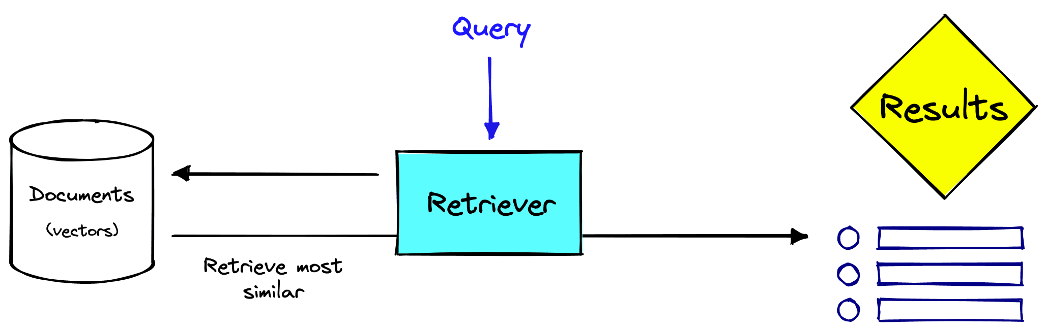
A single stage retrieval system. Note that the retriever may be sparse, dense, or even both.
A part of that is the research into more robust and learnable sparse embedding models — and one of the most performant models in this space is SPLADE.
The idea behind the Sparse Lexical and Expansion models is that a pretrained language model like BERT can identify connections between words/sub-words (called word-pieces or “terms” in this article) and use that knowledge to enhance our sparse vector embedding.
This works in two ways, it allows us to weigh the relevance of different terms (something like the will carry less relevance than a less common word like orangutan). And it enables term expansion: the inclusion of alternative but relevant terms beyond those found in the original sequence.
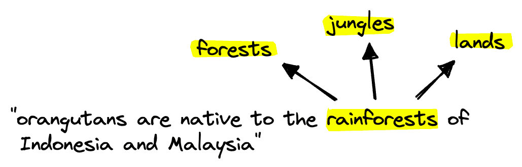
Term expansion allows us to identify relevant but different terms and use them in the sparse vector retrieval step.
The most significant advantage of SPLADE is not necessarily that it can do term expansion but instead that it can learn term expansions. Traditional methods required rule-based term expansion which is time-consuming and fundamentally limited. Whereas SPLADE can use the best language models to learn term expansions and even tweak them based on the sentence context.
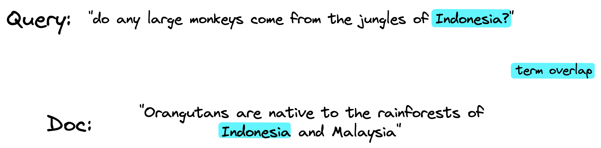
Despite having a query and document with many relevant terms, because they are not “exact matches” they are not identified.
Term expansion is crucial in minimizing the vocabulary mismatch problem — the typical lack of term overlap between queries and relevant documents.
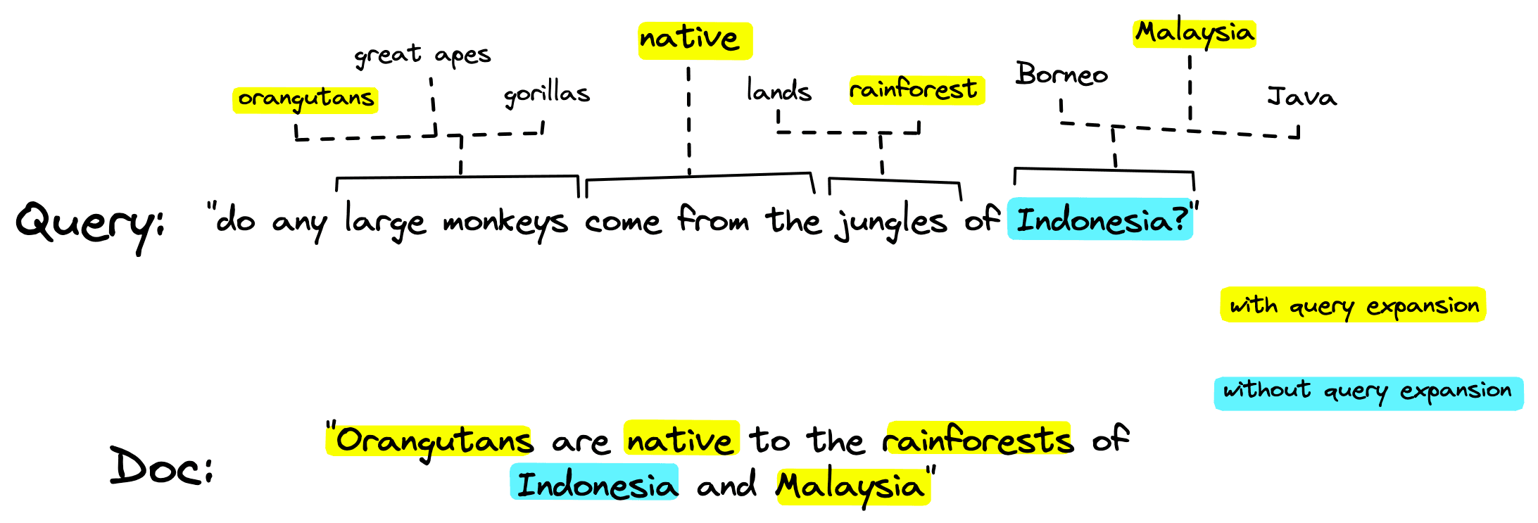
With term expansion on our query we will a much larger overlap because we’re now able to identify similar words.
It’s expected that relevant documents can contain little-to-no term overlap because of the complexity of language and the multitude of ways we can describe something.
How SPLADE builds its sparse embeddings is simple to understand. We start with a transformer model like BERT using a Masked-Language Modeling (MLM) head.
MLM is the typical pretraining method utilized by many transformers. We can start with an off-the-shelf pretrained BERT model.
As mentioned, we will use BERT with an MLM head. If you’re familiar with BERT and MLM, then great — if not, let’s break it down.
BERT is a popular transformer model. Like all transformers, its core functionality is to create information-rich token embeddings. What exactly does that mean?
We start with some text like "Orangutans are native to the rainforests of Indonesia and Malaysia". We would begin by tokenizing the text into BERT-specific sub-word tokens:
In[2]:
text = (
    "Orangutans are native to the rainforests of "
    "Indonesia and Malaysia"
)

# create the tokens that will be input into the model
tokens = tokenizer(text, return_tensors="pt")
tokens
Out[2]:
{'input_ids': tensor([[  101,  2030,  5654, 13210,  3619,  2024,  3128,  2000,  1996, 18951,
          2015,  1997,  6239,  1998,  6027,   102]]), 'token_type_ids': tensor([[0, 0, 0, 0, 0, 0, 0, 0, 0, 0, 0, 0, 0, 0, 0, 0]]), 'attention_mask': tensor([[1, 1, 1, 1, 1, 1, 1, 1, 1, 1, 1, 1, 1, 1, 1, 1]])}
In[3]:
# we transform the input_ids to human-readable tokens
tokenizer.convert_ids_to_tokens(tokens["input_ids"][0])
Out[3]:
['[CLS]',
 'or',
 '##ang',
 '##uta',
 '##ns',
 'are',
 'native',
 'to',
 'the',
 'rainforest',
 '##s',
 'of',
 'indonesia',
 'and',
 'malaysia',
 '[SEP]']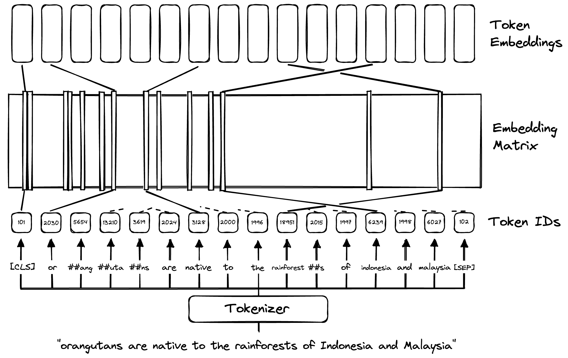
Token IDs are mapped to learned token embeddings within the embedding matrix.
These tokens are matched up to an “embedding matrix” that acts as the first layer in the BERT model. In this embedding matrix, we find learned “vector embeddings” that act as a “numerical representation” of these word/sub-word tokens.
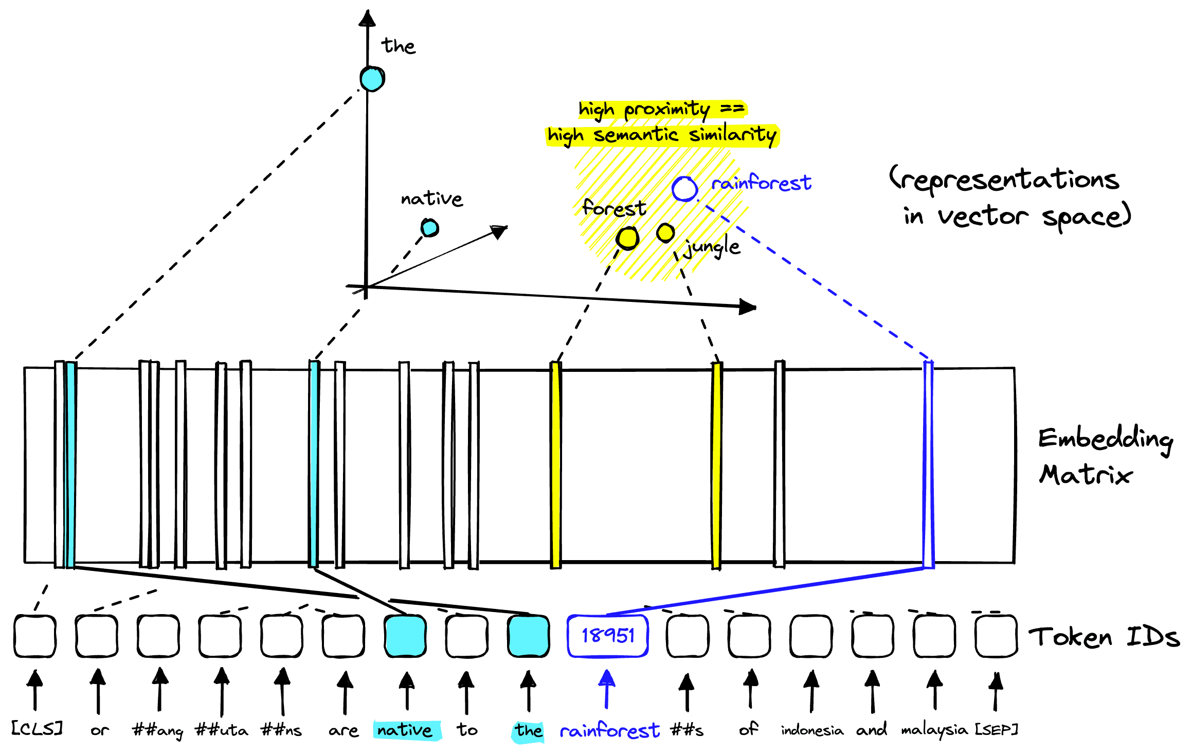
The vectors of the embedding matrix each represent a token within a meaningful vector space.
From here, the token representations of our original text go through several “encoder blocks”. These blocks encode more and more contextual information into each vector embedding based on the surrounding context from the rest of the text.
After this, we arrive at our transformer’s “output”, the information-rich vector embeddings. Each embedding represents the earlier token but with added information gathered from the other token vector embeddings also extracted from the original sentence.
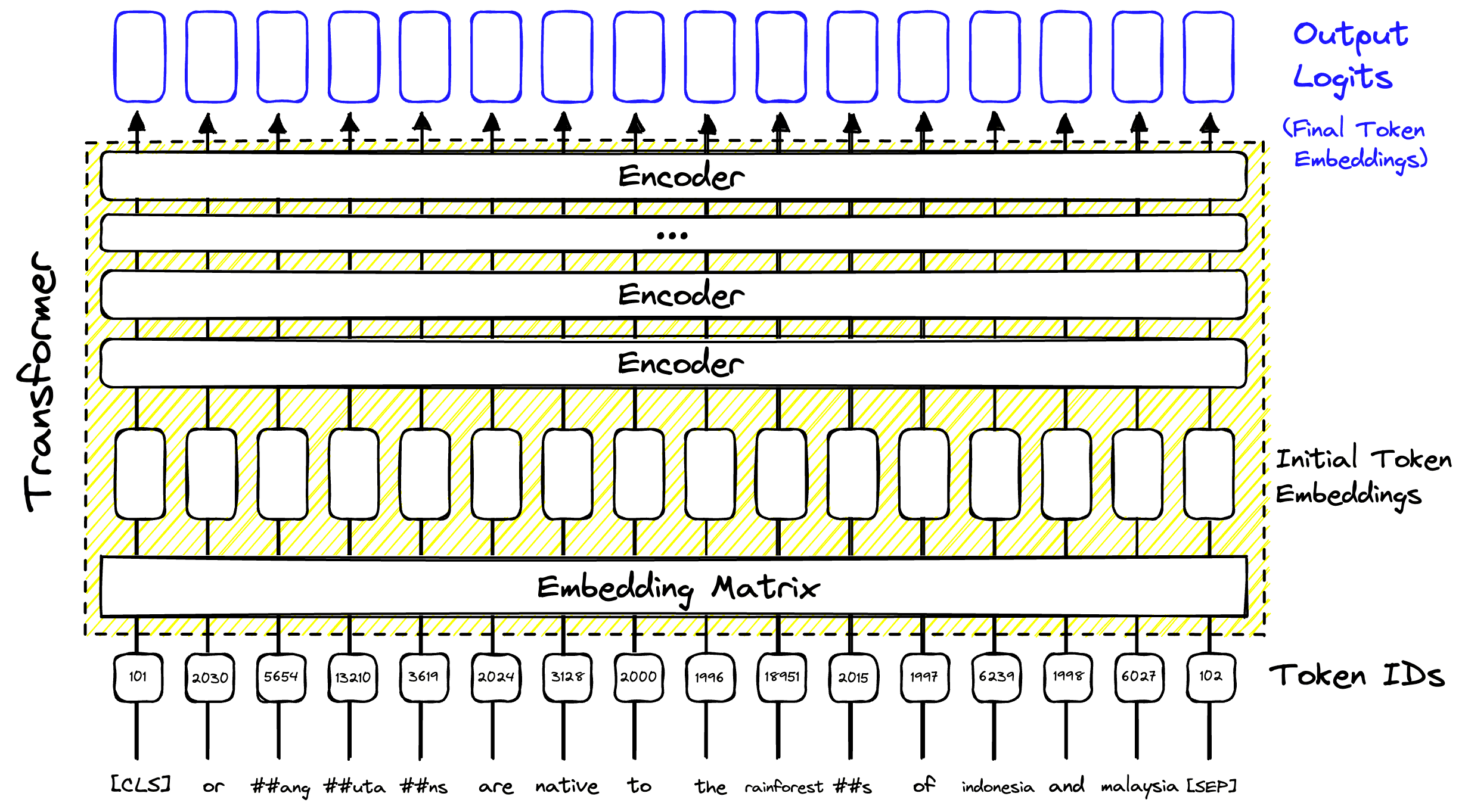
Processing the initial token embedding through several attention encoder blocks allows more contextual information to be encoded, producing information-rich embeddings.
This process is the core of BERT and every other transformer model. However, the power of transformers is the considerable number of things for which these information-rich vectors can be used. Typically, we add a task-specific “head” to a transformer to transform these vectors into something else, like predictions or sparse vectors.
The MLM head is one of many heads commonly used with BERT models. Unlike most heads, an MLM head is used during the initial pretraining of BERT.
This works by taking an input sentence; again, let’s use "Orangutans are native to the rainforests of Indonesia and Malaysia". We tokenize the text and then replace random tokens with a [MASK] token.
![Any word or sub-word token can be masked using the [MASK] token.](https://www.pinecone.io/_next/image/?url=https%3A%2F%2Fcdn.sanity.io%2Fimages%2Fvr8gru94%2Fproduction%2Fc42f70bc4a63b5ff24ac0eb763af20bdfe6d45fc-1770x363.png&w=3840&q=75)
Any word or sub-word token can be masked using the [MASK] token.
This masked token sequence is passed as input to BERT. At the other end, we give the original sentence to the MLM head. BERT and the MLM head are then optimized for predicting the original word/sub-word token that had been replaced by a [MASK] token.
![The MLM head produces a probability distribution from each output logit. The probabilities act as predictions of [MASK] representing each token from the vocab.](https://www.pinecone.io/_next/image/?url=https%3A%2F%2Fcdn.sanity.io%2Fimages%2Fvr8gru94%2Fproduction%2Fd64d431fb1b50ae9aa94b5cd85e1cdffe5eb7ca1-2318x1516.png&w=3840&q=75)
The MLM head produces a probability distribution from each output logit. The probabilities act as predictions of [MASK] representing each token from the vocab.
For this to work, the MLM head contains 30522 output values for each token position. These 30522 values represent the BERT vocabulary and act as a probability distribution over the vocab. The highest activation represents the token prediction for that particular token position.
These 30522 probability distributions act as an indicator of which words/tokens from the vocab are most important. The MLM head outputs these distributions for every token input to the model.
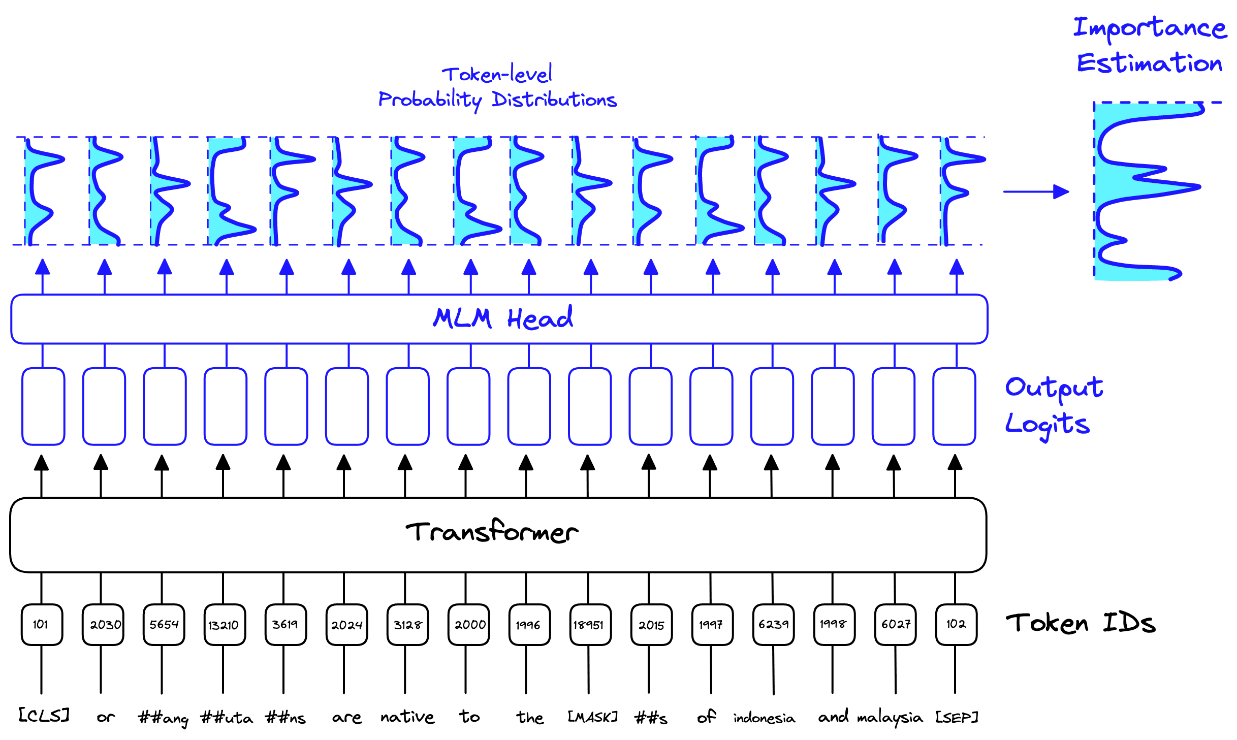
The MLM head gives us a probability distribution for each token, whether or not they have been masked. These distributions are aggregated to give the importance estimation.
SPLADE takes all these distributions and aggregates them into a single distribution called the importance estimation . This importance estimation is the sparse vector produced by SPLADE. We can combine all these probability distributions into a single distribution that tells us the relevance of every token in the vocab to our input sentence.
Where:
: Every token in the input set of tokens .
: Every predicted weight for all tokens in the vocab , for each token .
This allows us to identify relevant tokens that do not exist within the input sentence. For example, if we mask the word rainforest, we may return high predictions
for the words jungle, land, and forest. These words and their associated probabilities would then be represented in the SPLADE-built sparse vector.
This learned query/document expansion to include other relevant terms is a crucial advantage of SPLADE over traditional sparse methods. Helping us minimize the vocabulary mismatch problem based on learned relationships and term context.
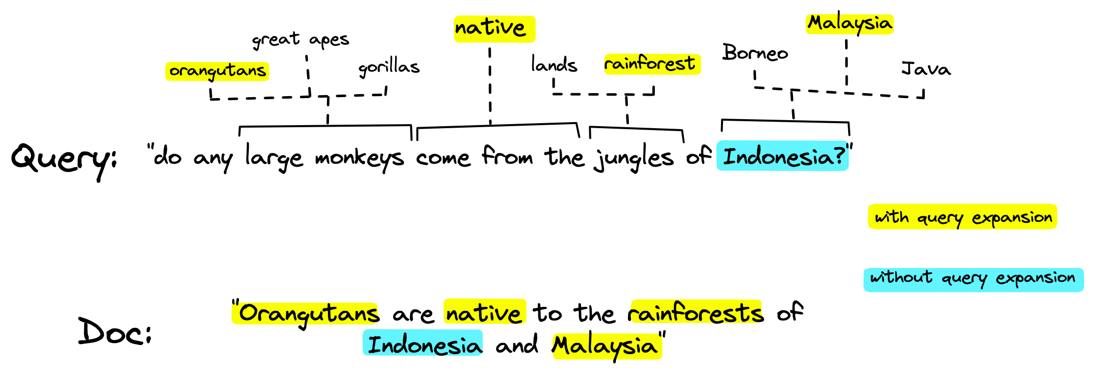
Term expansion in the query can lead to much greater overlap between queries and relevant documents, helping us minimize the vocabulary mismatch problem.
As many transformer models are pretrained with MLM, there are a large number of models that have trained MLM head weights that can be used for later SPLADE fine-tuning.
SPLADE is an excellent approach to minimizing the vocabulary mismatch problem commonly found in sparse vector methods. However, there are some drawbacks that we need to consider.
Compared to other sparse methods, retrieval with SPLADE is slow. There are three primary reasons for this:
Fortunately, there are solutions to all of these problems. For (1), the authors of SPLADE addressed this in a later version of the model that minimizes the number of query vector non-zero values [2].
Reducing the number of query vector non-zero values was made possible through two steps. First, by first improving the performance of the SPLADE document encodings via a max pooling modification to the original pooling strategy:
Second, by limiting term expansion to the document encodings only. Thanks to the improved document encoding performance, dropping query expansions still leaves us with better performance than the original SPLADE model.
Both (2) and (3) are solved using the Pinecone vector database. (2) is solved by Pinecone’s retrieval engine being designed from the ground up to be agnostic to data distribution. Pinecone allows real-valued sparse vectors — meaning SPLADE vectors are supported by default.
We have two options for implementing SPLADE; directly with Hugging Face transformers and PyTorch, or with more abstraction using the official SPLADE library. We will demonstrate both, starting with the Hugging Face and PyTorch implementation to understand how it works.
To begin, we install all prerequisites:
!pip install -U transformers torch
Then we initialize the BERT tokenizer and BERT model with masked-language modeling (MLM) head. We load the fine-tuned SPLADE model weights from naver/splade-cocondenser-ensembledistil.
from transformers import AutoModelForMaskedLM, AutoTokenizer

model_id = 'naver/splade-cocondenser-ensembledistil'

tokenizer = AutoTokenizer.from_pretrained(model_id)
model = AutoModelForMaskedLM.from_pretrained(model_id)
From here, we can create an input document text, tokenize it, and process it through the model to produce the MLM head output logits.
In[24]:
tokens = tokenizer(text, return_tensors='pt')
output = model(**tokens)
output
Out[24]:
MaskedLMOutput(loss=None, logits=tensor([[[ -6.9833,  -8.2131,  -8.1693,  ...,  -8.1552,  -7.8168,  -5.8152],
         [-13.6888, -11.7828, -12.5595,  ..., -12.4415, -11.5789, -12.0632],
         [ -8.7075,  -8.7019,  -9.0092,  ...,  -9.1933,  -8.4834,  -6.8165],
         ...,
         [ -5.1051,  -7.7245,  -7.0402,  ...,  -7.5713,  -6.9855,  -5.0462],
         [-23.5020, -18.8779, -17.7931,  ..., -18.2811, -17.2806, -19.4826],
         [-21.6329, -17.7142, -16.6525,  ..., -17.1870, -16.1865, -17.9581]]],
       grad_fn=<ViewBackward0>), hidden_states=None, attentions=None)
Out[25]:
torch.Size([1, 91, 30522])This leaves us with 91 probability distributions, each of dimensionality 30522. To transform this into the SPLADE sparse vector, we do the following:
In[26]:
import torch

vec = torch.max(
    torch.log(
        1 + torch.relu(output.logits)
    ) * tokens.attention_mask.unsqueeze(-1),
dim=1)[0].squeeze()

vec.shape
Out[27]:
tensor([0., 0., 0., ..., 0., 0., 0.], grad_fn=<SqueezeBackward0>)Because our vector is sparse, we can transform it into a much more compact dictionary format, keeping only the non-zero positions and weights.
In[29]:
# extract non-zero positions
cols = vec.nonzero().squeeze().cpu().tolist()
print(len(cols))

# extract the non-zero values
weights = vec[cols].cpu().tolist()
# use to create a dictionary of token ID to weight
sparse_dict = dict(zip(cols, weights))
sparse_dict
Out[29]:
{1000: 0.6246446967124939,
 1039: 0.45678916573524475,
 1052: 0.3088974058628082,
 1997: 0.15812619030475616,
 1999: 0.07194626331329346,
 2003: 0.6496524810791016,
 2024: 0.9411943554878235,
 ...,
 29215: 0.3594200909137726,
 29278: 2.276832342147827}
This is the final format of our sparse vector, but it’s not very interpretable. What we can do is translate the token ID keys to human-readable plaintext tokens. We do that like so:
In[28]:
# extract the ID position to text token mappings
idx2token = {
    idx: token for token, idx in tokenizer.get_vocab().items()
}
In[30]:
# map token IDs to human-readable tokens
sparse_dict_tokens = {
    idx2token[idx]: round(weight, 2) for idx, weight in zip(cols, weights)
}
# sort so we can see most relevant tokens first
sparse_dict_tokens = {
    k: v for k, v in sorted(
        sparse_dict_tokens.items(),
        key=lambda item: item[1],
        reverse=True
    )
}
sparse_dict_tokens
Out[30]:
{'pc': 3.02,
 'lace': 2.95,
 'programmed': 2.36,
 '##for': 2.28,
 'madagascar': 2.26,
 'death': 1.96,
 '##d': 1.95,
 'lattice': 1.81,
 ...,
 'carter': 0.0,
 'reg': 0.0}
Now we can see the most highly scored tokens from the sparse vector, including important field-specific terms like programmed, cell, lattice, regulated, and so on.
Another higher-level alternative is using the SPLADE library itself. We install it with pip install git+https://github.com/naver/splade.git and initialize the same model and vector building steps as above, using:
from splade.models.transformer_rep import Splade

sparse_model_id = 'naver/splade-cocondenser-ensembledistil'

sparse_model = Splade(sparse_model_id, agg='max')
sparse_model.eval()
We must still tokenize the input using a Hugging Face tokenizer to give us tokens, then we create the sparse vectors with:
In[13]:
with torch.no_grad():
    sparse_emb = naver_model(
        d_kwargs=tokens
    )['d_rep'].squeeze()
sparse_emb.shape
These embeddings can be processed into a smaller sparse vector dictionary using the same code above. The resultant data is the same as we built with the Hugging Face and PyTorch method.
Let’s look at how to actually compare our sparse vectors. We’ll define three short texts.
texts = [
   "Programmed cell death (PCD) is the regulated death of cells within an organism",
   "How is the scheduled death of cells within a living thing regulated?",
   "Photosynthesis is the process of storing light energy as chemical energy in cells"
]
As before, we encode everything with the tokenizer, build output logits with the model, and transform the token-level vectors into single sparse vectors.
In[15]:
tokens = tokenizer(
    texts, return_tensors='pt',
    padding=True, truncation=True
)
output = model(**tokens)
# aggregate the token-level vecs and transform to sparse
vecs = torch.max(
    torch.log(1 + torch.relu(output.logits)) * tokens.attention_mask.unsqueeze(-1), dim=1
)[0].squeeze().detach().cpu().numpy()
vecs.shape
We now have three 30522-dimensional sparse vectors. To compare them, we can use cosine or dot-product similarity. Using cosine similarity, we do the following:
In[16]:
import numpy as np

sim = np.zeros((vecs.shape[0], vecs.shape[0]))

for i, vec in enumerate(vecs):
    sim[i,:] = np.dot(vec, vecs.T) / (
        np.linalg.norm(vec) * np.linalg.norm(vecs, axis=1)
    )
Out[17]:
array([[1.        , 0.54609376, 0.20535842],
       [0.54609376, 0.99999988, 0.20411882],
       [0.2053584 , 0.20411879, 1.        ]])
Leaving us with:
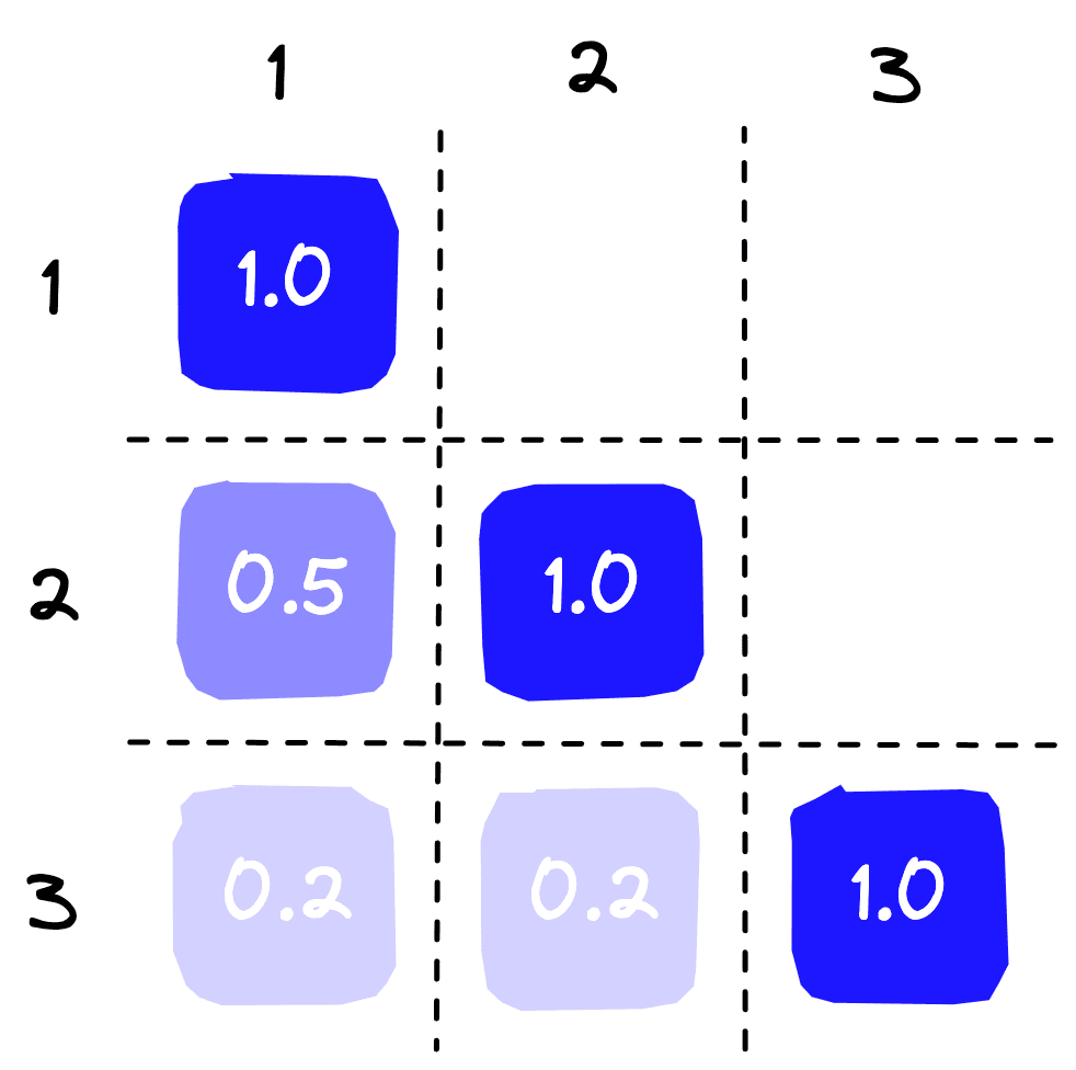
Similarity heatmap using calculated values from sim above. Sentences 1 and 2 share the highest similarity (with the exception of the diagonals which are just a comparison of each sentence to itself).
The two similar sentences naturally score higher than the third irrelevant sentence.
That’s it for this introduction to learned sparse embeddings with SPLADE. Through SPLADE, we can represent text with efficient sparse vector embeddings. Helping us deal with the vocabulary mismatch problem while enabling exact matching.
We’ve also seen where SPLADE falls short when used in traditional retrieval systems. Fortunately, we covered how improvements through SPLADEv2 and distribution agnostic retrieval systems like Pinecone can help us sidestep those shortfalls.
There is still plenty more to be done. More research and recent efforts demonstrate the benefit of mixing both dense and sparse representations using hybrid search indexes. In this, and many other advances, we can see vector search becoming ever more accurate and accessible.
[1] T. Formal, B. Piwowarski, S. Clinchant, SPLADE: Sparse Lexical and Expansion Model for First Stage Ranking (2021), SIGIR 21
[2] T. Formal, C. Lassance, B. Piwowarski, S. Clinchant, SPLADE v2: Sparse Lexical and Expansion Model for Information Retrieval (2021)
此内容由惯性聚合(RSS阅读器)自动聚合整理,仅供阅读参考。 原文来自 — 版权归原作者所有。