







Industries today deal with ever increasing amounts of data. Especially in retail, fashion, and other industries where the image representation of products plays an important role.
In such a situation, we can often describe one product in many ways, making it challenging to perform accurate and least time-consuming searches.
Could I take advantage of state-of-the-art artificial intelligence solutions to tackle such a challenge?
This is where OpenAI’s CLIP comes in handy. A deep learning algorithm that makes it easy to connect text and images.
After completing this conceptual blog, you will understand: (1) what CLIP is, (2) how it works and why you should adopt it, and finally, (3) how to implement it for your own use case using both local and cloud-based vector indexes.
Contrastive Language-Image Pre-training (CLIP for short) is a state-of-the-art model introduced by OpenAI in February 2021 [1].
CLIP is a neural network trained on about 400 million (text and image) pairs. Training uses a contrastive learning approach that aims to unify text and images, allowing tasks like image classification to be done with text-image similarity.
This means that CLIP can find whether a given image and textual description match without being trained for a specific domain. Making CLIP powerful for out-of-the-box text and image search, which is the main focus of this article.
Besides text and image search, we can apply CLIP to image classification, image generation, image similarity search, image ranking, object tracking, robotics control, image captioning, and more.
Below are some reasons that increased the adoption of the CLIP models by the AI community
The use of the contrastive objective increased the efficiency of the CLIP model by 4-to-10x more at zero-shot ImageNet classification.
Also, the adoption of the Vision Transformer created an additional 3x gain in compute efficiency compared to the standard ResNet.
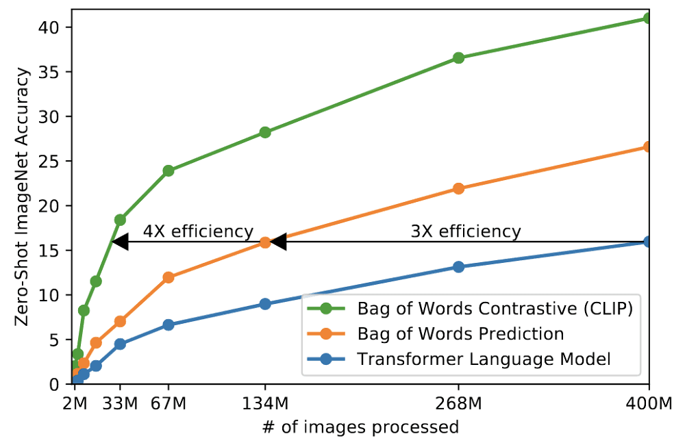
The efficiency of CLIP at zero-shot transfer
CLIP outperforms existing ImageNet models in new domains because of its ability to learn a wide range of visual representations directly from natural language.
The following graphic highlights CLIP zero-shot performance compared to ResNet models few-shot linear probe performance on fine-grained object detection, geo-localization, action recognition, and optical character recognition tasks.
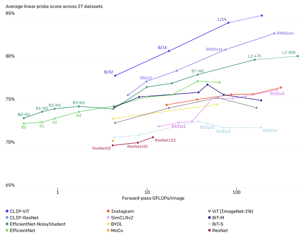
Average linear probe score across 27 datasets
CLIP architecture consists of two main components: (1) a text encoder, and (2) an Image encoder. These two encoders are jointly trained to predict the correct pairings of a batch of training (image, text) examples.
We can answer this question by understanding these three approaches: (1) contrastive pre-training, (2) dataset classifier creation from labeled text, and finally, (3) application of the zero-shot technique for classification.
Let’s explain each of these three concepts.
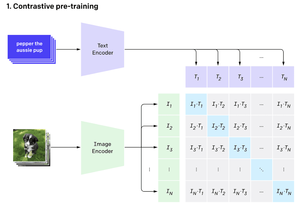
Contrastive pre-training
During this phase, a batch of 32,768 pairs of image and text is passed through the text and image encoders simultaneously to generate the vector representations of the text and the associated image, respectively.
The training is done by searching for each image, the closest text representation across the entire batch, which corresponds to maximizing cosine similarity between the actual N pairs that are maximally close.
Also, it makes the actual images far away from all the other texts by minimizing their cosine similarity.
Finally, a symmetric cross-entropy loss is optimized over the previously computed similarity scores.

Classification dataset creation and zero-shot prediction
This second step section encodes all the labels/objects in the following context format: “a photo of a {object}. The vector representation of each context is generated from the text encoder.
If we have dog, car, and plane as the classes of the dataset, we will output the following context representations:
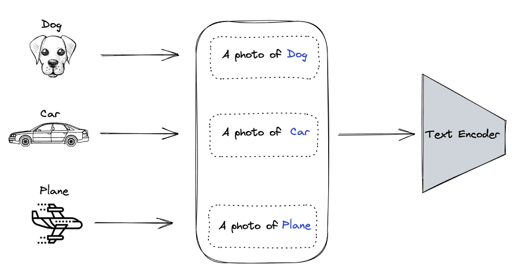
Image illustration of the context representations
We use the output of section 2 to predict which image vector corresponds to which context vector. The benefit of applying the zero-shot prediction approach is to make CLIP models generalize better on unseen data.
Now that we know the architecture of CLIP and how it works, this section will walk you through all the steps to successfully implement two real-world scenarios. First, you will understand how to perform an image search in natural language. Also, you will be able to perform an image-to-image search using.
At the end of the process, you will understand the benefits of using a vector database for such a use case.
(Follow along with the Colab notebook!)
The end-to-end process is explained through the workflow below. We start by collecting data from the Hugging Face dataset, which is then processed to further generate vector index vectors through the Image and Text Encoders. Finally, the Pinecone client is used to insert them to a vector index.
The user will then be able to search images based on either text or another image.
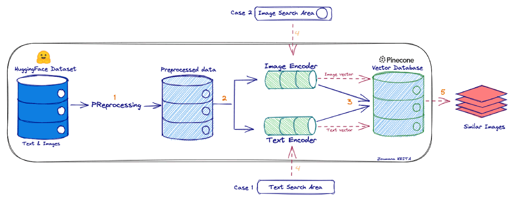
General workflow for image search
The following libraries are required to create the implementation.
%%bash
# Uncomment this if using it for the first time. -qqq for ZERO-OUT
pip3 -qqq install transformers torch datasets

# The following two libraries avoid the UnidentifiedImageError
pip3 -qqq install gdcm
pip3 -qqq install pydicom
pip -qqq install faiss-gpu
pip -qqq install pinecone-clientimport os
import faiss
import torch
import skimage
import requests
import pinecone
import numpy as np
import pandas as pd
from PIL import Image
from io import BytesIO
import IPython.display
import matplotlib.pyplot as plt
from datasets import load_dataset
from collections import OrderedDict
from transformers import CLIPProcessor, CLIPModel, CLIPTokenizerThe conceptual captions dataset consists of around 3.3M images with two main columns: the image URL and its caption. You can find more details from the corresponding huggingface link.
# Get the dataset
image_data = load_dataset("conceptual_captions", split="train")Not all URLs in the dataset are valid. We fix that by testing and removing all erroneous URL entries.
def check_valid_URLs(image_URL):
   try:
     response = requests.get(image_URL)
     Image.open(BytesIO(response.content))
     return True
   except:
     return False
def get_image(image_URL):
   response = requests.get(image_URL)
   image = Image.open(BytesIO(response.content)).convert("RGB")
   return image
The following expression creates a new dataframe with a new column “is_valid” which is True when the URL is valid or False otherwise.
# Transform dataframe
image_data_df["is_valid"] = image_data_df["image_url"].apply(check_valid_URLs)
# Get valid URLs
image_data_df = image_data_df[image_data_df["is_valid"]==True]
# Get image from URL
image_data_df["image"] = image_data_df["image_url"].apply(get_image)
The second step is to download the images from the URLs. This helps us avoid constant web requests.
The prerequisites to successfully implement the encoders are the model, the processor, and the tokenizer.
The following function fulfills those requirements from the model ID and the device used for the computation, either CPU or GPU.
def get_model_info(model_ID, device):
# Save the model to device
	model = CLIPModel.from_pretrained(model_ID).to(device)
 	# Get the processor
	processor = CLIPProcessor.from_pretrained(model_ID)
# Get the tokenizer
	tokenizer = CLIPTokenizer.from_pretrained(model_ID)
       # Return model, processor & tokenizer
	return model, processor, tokenizer
# Set the device
device = "cuda" if torch.cuda.is_available() else "cpu"
# Define the model ID
model_ID = "openai/clip-vit-base-patch32"
# Get model, processor & tokenizer
model, processor, tokenizer = get_model_info(model_ID, device)We start by generating the embedding of a single text before applying the same function across the entire dataset.
def get_single_text_embedding(text):
inputs = tokenizer(text, return_tensors = "pt")
	text_embeddings = model.get_text_features(**inputs)
 	# convert the embeddings to numpy array
	embedding_as_np = text_embeddings.cpu().detach().numpy()
return embedding_as_np
def get_all_text_embeddings(df, text_col):
df["text_embeddings"] = df[str(text_col)].apply(get_single_text_embedding)
return df
# Apply the functions to the dataset
image_data_df = get_all_text_embeddings(image_data_df, "caption")
The first five rows look like this:

Format of the vector index containing the captions/text embeddings
The same process is used for image embeddings but with different functions.
def get_single_image_embedding(my_image):
image = processor(
		text = None,
		images = my_image,
		return_tensors="pt"
		)["pixel_values"].to(device)
embedding = model.get_image_features(image)
# convert the embeddings to numpy array
	embedding_as_np = embedding.cpu().detach().numpy()
	return embedding_as_np
 def get_all_images_embedding(df, img_column):
	df["img_embeddings"] = df[str(img_column)].apply(get_single_image_embedding)
	return df
image_data_df = get_all_images_embedding(image_data_df, "image")
The final format of the text and image vector index looks like this:
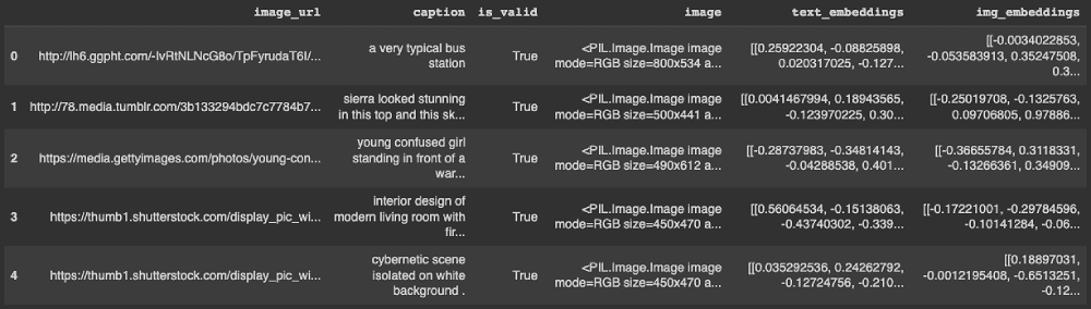
Vector index with image and captions embeddings (Image by Author)
In this section, we will explore two different approaches to storing the embeddings and metadata for performing the searches: The first is using the previous dataframe, and the second is using Pinecone. Both approaches use the cosine similarity metric.
The helper function get_top_N_images generates similar images for the two scenarios illustrated in the workflow above: text-to-image search or image-to-image search.
from sklearn.metrics.pairwise import cosine_similarity
def get_top_N_images(query, data, top_K=4, search_criterion="text"):
   # Text to image Search
   if(search_criterion.lower() == "text"):
     query_vect = get_single_text_embedding(query)
   # Image to image Search
   else:
     query_vect = get_single_image_embedding(query)
   # Relevant columns
   revevant_cols = ["caption", "image", "cos_sim"]
   # Run similarity Search
   data["cos_sim"] = data["img_embeddings"].apply(lambda x: cosine_similarity(query_vect, x))# line 17
   data["cos_sim"] = data["cos_sim"].apply(lambda x: x[0][0])
   """
   Retrieve top_K (4 is default value) articles similar to the query
   """
  most_similar_articles = data.sort_values(by='cos_sim',  ascending=False)[1:top_K+1] # line 24
   return most_similar_articles[revevant_cols].reset_index()
Let’s understand how we perform the recommendation.
→ The user provides either a text or an image as a search criterion, but the model performs a text-to-image search by default.
→ In line 17, a cosine similarity is performed between each image vector and the user’s input vector.
→ Finally, in line 24, sort the result based on the similarity score in descending order, and we return the most similar images by excluding the first one corresponding to the query itself.
This helper function makes it easy to have a side-by-side visualization of the recommended images. Each image will have the corresponding caption and similarity score.
def plot_images_by_side(top_images):
 index_values = list(top_images.index.values)
 list_images = [top_images.iloc[idx].image for idx in index_values]
 list_captions = [top_images.iloc[idx].caption for idx in index_values]
 similarity_score = [top_images.iloc[idx].cos_sim for idx in index_values]
 n_row = n_col = 2
 _, axs = plt.subplots(n_row, n_col, figsize=(12, 12))
 axs = axs.flatten()
 for img, ax, caption, sim_score in zip(list_images, axs, list_captions, similarity_score):
     ax.imshow(img)
     sim_score = 100*float("{:.2f}".format(sim_score))
     ax.title.set_text(f"Caption: {caption}\nSimilarity: {sim_score}%")
plt.show()→ First, the user provides the text that is used for the search.
→ Second, we run a similarity search.
→ Third, we plot the images recommended by the algorithm.
query_caption = image_data_df.iloc[10].caption
# Print the original query text
print("Query: {}".format(query_caption))
# Run the similarity search
top_images = get_top_N_images(query_caption, image_data_df)
# Plot the recommended images
plot_images_by_side(top_images)
Line 3 generates the following text:
Query: actor arrives for the premiere of the film
Line 9 produces the plot below.
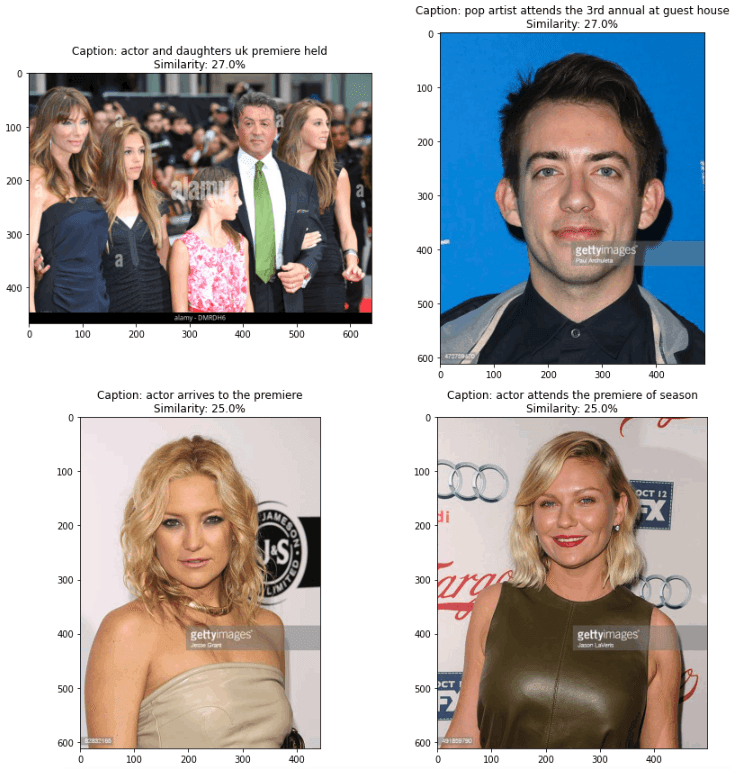
Images corresponding to the text: “actor arrives for the premiere of the film”
The same process applies. The only difference this time is that the user provides an image instead of a caption.
# Get the query image and show it
query_image = image_data_df.iloc[55].image
query_image
Original image of search (image at the index)
# Run the similarity search and plot the result
top_images = get_top_N_images(query_image, image_data_df, search_criterion="image")
# Plot the result
plot_images_by_side(top_images)
We run the search by specifying the search_criterion which is “image” in line 2.
The final result is shown below.

Images corresponding to the image-to-image search (Image by Author)
We can observe that some of the images are less similar which introduces noise in the recommendation. We can reduce that noise by specifying a threshold level of similarity. For instance, consider all the images with at least 60% similarity.
Pinecone provides a fully-managed, easily scalable vector database that makes it easy to build high-performance vector search applications.
This section will walk you through the steps from acquiring your API credentials to implementing the search engine.
Below are the eight steps to acquire your API credentials, starting from the Pinecone website.
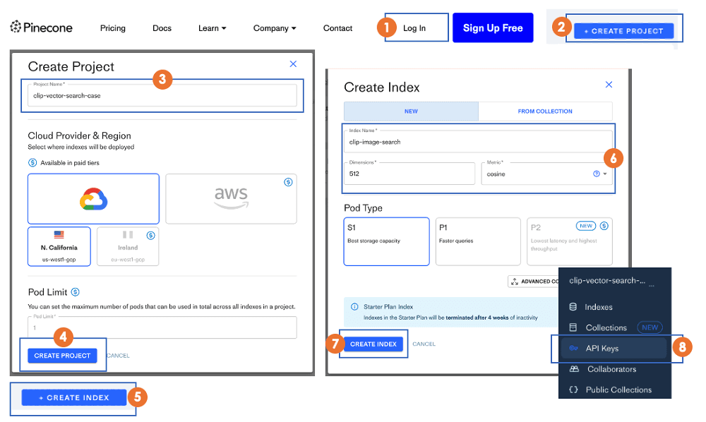
Eight main steps to acquire your Pinecone Client API
From the API, we can create the index that allows us to perform all the create, update, delete, and insert actions.
pinecone.init(
   api_key = "YOUR_API_KEY",
   environment="YOUR_ENV"  # find next to API key in console
)
my_index_name = "clip-image-search"
vector_dim = image_data_df.img_embeddings[0].shape[1]

if my_index_name not in pinecone.list_indexes():
 # Create the vectors dimension
 pinecone.create_index(name = my_index_name,
                       dimension=vector_dim,
                       metric="cosine", shards=1,
                       pod_type='s1.x1')
# Connect to the index
my_index = pinecone.Index(index_name = my_index_name)The result of the following instruction shows that we have no data in the index.
my_index.describe_index_stats()The only information we have is the dimension, which is 512.
{'dimension': 512,
           'index_fullness': 0.0,
            'namespaces': {},
'total_vector_count': 0}Now that we have configured the Pinecone database, the next step is to populate it with the following code.
image_data_df["vector_id"] = image_data_df.index
image_data_df["vector_id"] = image_data_df["vector_id"].apply(str)
# Get all the metadata
final_metadata = []
for index in range(len(image_data_df)):
 final_metadata.append({
     'ID':  index,
     'caption': image_data_df.iloc[index].caption,
     'image': image_data_df.iloc[index].image_url
 })
image_IDs = image_data_df.vector_id.tolist()
image_embeddings = [arr.tolist() for arr in image_data_df.img_embeddings.tolist()]
# Create the single list of dictionary format to insert
data_to_upsert = list(zip(image_IDs, image_embeddings, final_metadata))
# Upload the final data
my_index.upsert(vectors = data_to_upsert)
# Check index size for each namespace
my_index.describe_index_stats()
Let’s understand what is going on here.
The data to upsert requires three components: the unique identifiers (IDs) of each observation, the list of embeddings being stored, and the metadata containing additional information about the data to store.
→ From lines 5 to 12, the metadata is created by storing the “ID”, “caption” and “URL” of each observation.
→ On lines 14 and 15, we generate a list of IDs, and convert the embeddings into a list of lists.
→ Then, we create a list of dictionaries mapping the IDs, embeddings, and metadata.
→ The final data is upserted to the index with the .upsert() function.
Similarly to the previous scenario, we can check that all vectors have been upserted via my_index.describe_index_stats().
All that remains is to query our index using the text-to-image and image-to-image searches. Both will use the following syntax:
my_index.query(my_query_embedding, top_k=N, include_metadata=True)→ my_query_embedding is the embedding (as a list) of the query (caption or image) provided by the user.
→ N corresponds to the top number of results to return.
→ include_metadata=True means that we want the query result to include metadata.
# Get the query text
text_query = image_data_df.iloc[10].caption

# Get the caption embedding
query_embedding = get_single_text_embedding(text_query).tolist()

# Run the query
my_index.query(query_embedding, top_k=4, include_metadata=True)
Below is the JSON response returned from the query
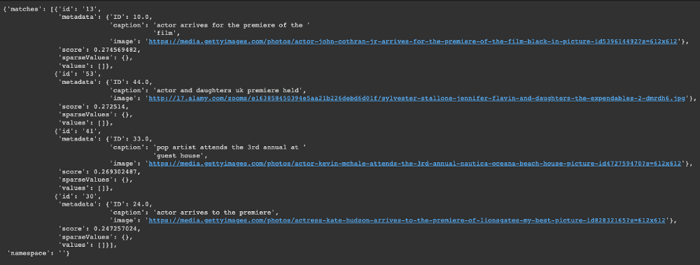
text-to-image query result (Image by Author)
From the “matches” attribute, we can observe the top four most similar images returned by the query.
The same approach applies to image-to-image search.
image_query = image_data_df.iloc[43].imageThis is the image provided by the user as the search criteria.

Query image
# Get the text embedding
query_embedding = get_single_image_embedding(image_query).tolist()

# Run the query
my_index.query(query_embedding, top_k=4, include_metadata=True)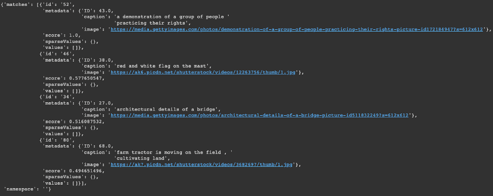
image-to-image query result (Image by Author)
Once you’ve finished don’t forget to delete your index to free up your resources with:
pinecone.delete_index(my_index)This approach using Pinecone has several advantages:
→ Simplicity: the querying approach is much simpler than the first approach, where the user has the full responsibility of managing the vector index.
→ Speed: Pinecone approach is faster, which corresponds to most industry requirements.
→ Scalability: vector index hosted on Pinecone is scalable with little-to-no user effort from us. The first approach would become increasingly complex and slow as we scale.
→ Lower chance of information loss: the vector index based on Pinecone is hosted in the cloud with backups and high information security. The first approach is too high risk for production use-cases.
→ Web-service friendly: the result provided by the query is in JSON format and can be consumed by other applications, making it a better fit for web-based applications.
Congratulations, you have just learned how to fully implement an image search application using both image and natural language. I hope the benefits highlighted are valid enough to take your project to the next level using vector databases.
Multiple resources are available at our Learning Center to further your learning.
The source code for the article is available here.
[1] A. Radford, J. W. Kim, et al., Learning Transferable Visual Models From Natural Language Supervision (2021)
[2] A. Vaswani, et al., Attention Is All You Need (2017), NeurIPS
此内容由惯性聚合(RSS阅读器)自动聚合整理,仅供阅读参考。 原文来自 — 版权归原作者所有。