







Transformer-produced sentence embeddings have come a long way in a very short time. Starting with the slow but accurate similarity prediction of BERT cross-encoders, the world of sentence embeddings was ignited with the introduction of SBERT in 2019 [1]. Since then, many more sentence transformers have been introduced. These models quickly made the original SBERT obsolete.
How did these newer sentence transformers manage to outperform SBERT so quickly? The answer is multiple negatives ranking (MNR) loss.
This article will cover what MNR loss is, the data it requires, and how to implement it to fine-tune our own high-quality sentence transformers.
Implementation will cover two training approaches. The first is more involved, and outlines the exact steps to fine-tune the model. The second approach makes use of the sentence-transformers library’s excellent utilities for fine-tuning.
NLI Training
As explained in our article on softmax loss, we can fine-tune sentence transformers using Natural Language Inference (NLI) datasets.
These datasets contain many sentence pairs, some that imply each other, and others that do not imply each other. As with the softmax loss article, we will use two of these datasets: the Stanford Natural Language Inference (SNLI) and Multi-Genre NLI (MNLI) corpora.
These two corpora total to 943K sentence pairs. Each pair consists of a premise and hypothesis sentence, which are assigned a label:
- 0 — entailment, e.g. the
premisesuggests thehypothesis. - 1 — neutral, the
premiseandhypothesiscould both be true, but they are not necessarily related. - 2 — contradiction, the
premiseandhypothesiscontradict each other.
When fine-tuning with MNR loss, we will be dropping all rows with neutral or contradiction labels — keeping only the positive entailment pairs.
We will be feeding sentence A (the premise, known as the anchor) followed by sentence B (the hypothesis, when the label is 0, this is called the positive) into BERT on each step. Unlike softmax loss, we do not use the label feature.
These training steps are performed in batches. Meaning several anchor-positive pairs are processed at once.
The model is then optimized to produce similar embeddings between pairs while maintaining different embeddings for non-pairs. We will explain this in more depth soon.
Data Preparation
Let’s look at the data preparation process. We first need to download and merge the two NLI datasets. We will use the datasets library from Hugging Face.
In[1]:
import datasets

snli = datasets.load_dataset('snli', split='train')
mnli = datasets.load_dataset('glue', 'mnli', split='train')

snli = snli.cast(mnli.features)

dataset = datasets.concatenate_datasets([snli, mnli])

del snli, mnli
Because we are using MNR loss, we only want anchor-positive pairs. We can apply a filter to remove all other pairs (including erroneous -1 labels).
In[2]:
print(f"before: {len(dataset)} rows")
dataset = dataset.filter(
    lambda x: True if x['label'] == 0 else False
)
print(f"after: {len(dataset)} rows")
Out[2]:
100%|██████████| 943/943 [00:17<00:00, 53.31ba/s]The dataset is now prepared differently depending on the training method we are using. We will continue preparation for the more involved PyTorch approach. If you’d rather just train a model and care less about the steps involved, feel free to skip ahead to the next section.
For the PyTorch approach, we must tokenize our own data. To do that, we will be using a BertTokenizer from the transformers library and applying the map method on our dataset.
In[3]:
from transformers import BertTokenizer

tokenizer = BertTokenizer.from_pretrained('bert-base-uncased')

dataset = dataset.map(
    lambda x: tokenizer(
            x['premise'], max_length=128, padding='max_length',
            truncation=True
        ), batched=True
)

dataset = dataset.rename_column('input_ids', 'anchor_ids')
dataset = dataset.rename_column('attention_mask', 'anchor_mask')

dataset
Out[3]:
Dataset({
    features: ['anchor_mask', 'hypothesis', 'anchor_ids', 'label', 'premise', 'token_type_ids'],
    num_rows: 314315
})
Encode `hypothesis` encodings.In[4]:
dataset = dataset.map(
    lambda x: tokenizer(
            x['hypothesis'], max_length=128, padding='max_length',
            truncation=True
    ), batched=True
)

dataset = dataset.rename_column('input_ids', 'positive_ids')
dataset = dataset.rename_column('attention_mask', 'positive_mask')

dataset = dataset.remove_columns(['premise', 'hypothesis', 'label', 'token_type_ids'])

dataset
Out[4]:
Dataset({
    features: ['anchor_ids', 'anchor_mask', 'positive_mask', 'positive_ids'],
    num_rows: 314315
})
After that, we’re ready to initialize our DataLoader, which will be used for loading batches of data into our model during training.
In[5]:
dataset.set_format(type='torch', output_all_columns=True)In[6]:
import torch

batch_size = 32

loader = torch.utils.data.DataLoader(dataset, batch_size=batch_size)
And with that, our data is ready. Let’s move on to training.
PyTorch Fine-Tuning
When training SBERT models, we don’t start from scratch. Instead, we begin with an already pretrained BERT — all we need to do is fine-tune it for building sentence embeddings.
from transformers import BertModel

# start from a pretrained bert-base-uncased model
model = BertModel.from_pretrained('bert-base-uncased')
MNR and softmax loss training approaches use a * ‘siamese’*-BERT architecture during fine-tuning. Meaning that during each step, we process a sentence A (our anchor) into BERT, followed by sentence B (our positive).
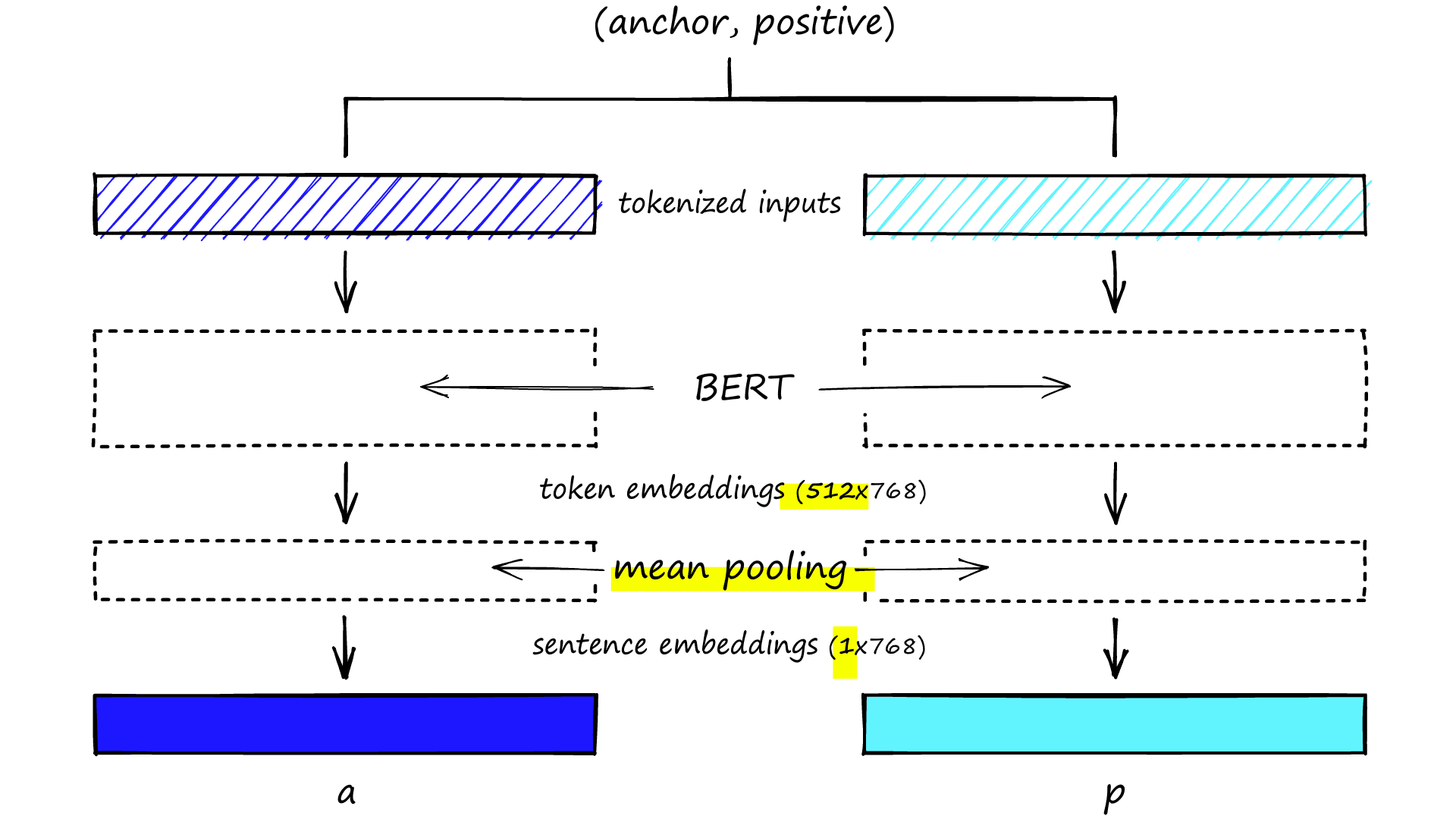
Siamese-BERT network, the anchor and positive sentence pairs are processed separately. A mean pooling layer converts token embeddings into sentence embeddings.sentence A is our anchor and sentence B the positive.
Because these two sentences are processed separately, it creates a siamese-like network with two identical BERTs trained in parallel. In reality, there is only a single BERT being used twice in each step.
We can extend this further with triplet-networks. In the case of triplet networks for MNR, we would pass three sentences, an anchor, it’s positive, and it’s negative. However, we are not using triplet-networks, so we have removed the negative rows from our dataset (rows where label is 2).
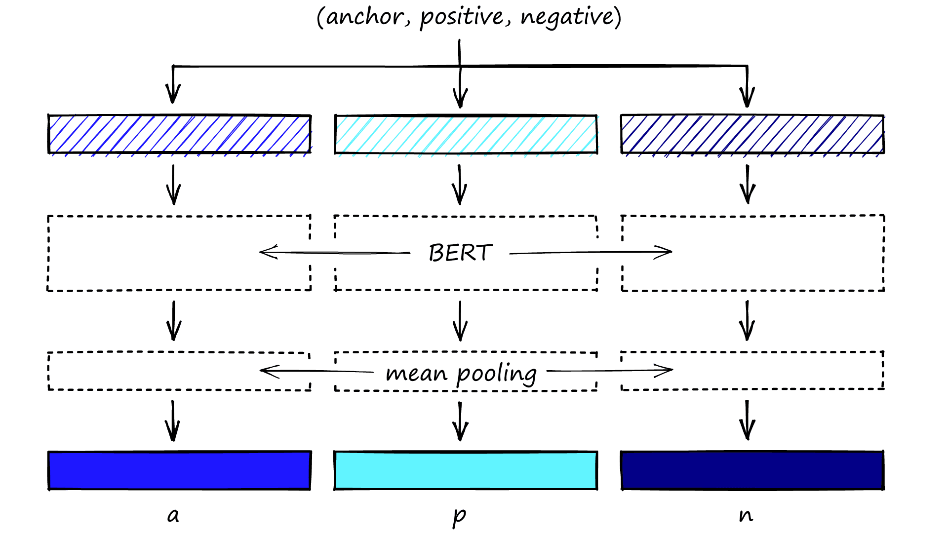
Triplet networks use the same logic but with an added sentence. For MNR loss this other sentence is the negative pair of the anchor.
BERT outputs 512 768-dimensional embeddings. We convert these into averaged sentence embeddings using mean-pooling. Using the siamese approach, we produce two of these per step — one for the anchor that we will call a, and another for the positive called p.
# define mean pooling function
def mean_pool(token_embeds, attention_mask):
    # reshape attention_mask to cover 768-dimension embeddings
    in_mask = attention_mask.unsqueeze(-1).expand(
        token_embeds.size()
    ).float()
    # perform mean-pooling but exclude padding tokens (specified by in_mask)
    pool = torch.sum(token_embeds * in_mask, 1) / torch.clamp(
        in_mask.sum(1), min=1e-9
    )
    return pool
In the mean_pool function, we’re taking these token-level embeddings (the 512) and the sentence attention_mask tensor. We resize the attention_mask to match the higher 768-dimensionality of the token embeddings.
The resized mask in_mask is applied to the token embeddings to exclude padding tokens from the mean pooling operation. Mean-pooling takes the average activation of values across each dimension but excluding those padding values, which would reduce the average activation. This operation transformers our token-level embeddings (shape 512*768) to sentence-level embeddings (shape 1*768).
These steps are performed in batches, meaning we do this for many (anchor, positive) pairs in parallel. That is important in our next few steps.
In[20]:
a.shape # check shape of batched inputs (batch_size == 32)First, we calculate the cosine similarity between each anchor embedding (a) and all of the positive embeddings in the same batch (p).
In[23]:
# define cosine sim layer
cos_sim = torch.nn.CosineSimilarity()
In[24]:
scores = []
for a_i in a:
    scores.append(cos_sim(a_i.reshape(1, a_i.shape[0]), p))
In[25]:
scores = torch.stack(scores)
scores
Out[25]:
tensor([[0.7799, 0.3883, 0.7147,  ..., 0.7094, 0.7934, 0.6639],
        [0.6685, 0.5236, 0.6153,  ..., 0.6807, 0.7095, 0.6229],
        [0.7462, 0.4453, 0.8049,  ..., 0.7482, 0.8092, 0.5914],
        ...,
        [0.7298, 0.4693, 0.6516,  ..., 0.8444, 0.8349, 0.6369],
        [0.7391, 0.4418, 0.7139,  ..., 0.8012, 0.9189, 0.6312],
        [0.7391, 0.4418, 0.7139,  ..., 0.8012, 0.9189, 0.6312]],
       device='cuda:0', grad_fn=<StackBackward>)
From here, we produce a vector of cosine similarity scores (of size batch_size) for each anchor embedding a_i (or size 2 * batch_size for triplets). Each anchor should share the highest score with its positive pair, p_i.
Cosine similarity scores using five pairs/triples in a triplet network (with (a, p, n)). A siamese network is the same but excluding the dark blue n blocks (n).
To optimize for this, we use a set of increasing label values to mark where the highest score should be for each a_i, and categorical cross-entropy loss.
In[27]:
labels = torch.tensor(range(len(scores)), dtype=torch.long, device=scores.device)
labels
Out[27]:
tensor([ 0,  1,  2,  3,  4,  5,  6,  7,  8,  9, 10, 11, 12, 13, 14, 15, 16, 17,
        18, 19, 20, 21, 22, 23, 24, 25, 26, 27, 28, 29, 30, 31],
       device='cuda:0')
In[28]:
# define loss function
loss_func = torch.nn.CrossEntropyLoss()
In[29]:
loss_func(scores, labels)Out[29]:
tensor(3.3966, device='cuda:0', grad_fn=<NllLossBackward>)And that’s every component we need for fine-tuning with MNR loss. Let’s put that all together and set up a training loop. First, we move our model and layers to a CUDA-enabled GPU if available.
In[30]:
# set device and move model there
device = torch.device('cuda') if torch.cuda.is_available() else torch.device('cpu')
model.to(device)
print(f'moved to {device}')
In[31]:
# define layers to be used in multiple-negatives-ranking
cos_sim = torch.nn.CosineSimilarity()
loss_func = torch.nn.CrossEntropyLoss()
scale = 20.0  # we multiply similarity score by this scale value
# move layers to device
cos_sim.to(device)
loss_func.to(device)
Then we set up the optimizer and schedule for training. We use an Adam optimizer with a linear warmup for 10% of the total number of steps.
In[32]:
from transformers.optimization import get_linear_schedule_with_warmup

# initialize Adam optimizer
optim = torch.optim.Adam(model.parameters(), lr=2e-5)

# setup warmup for first ~10% of steps
total_steps = int(len(anchors) / batch_size)
warmup_steps = int(0.1 * total_steps)
scheduler = get_linear_schedule_with_warmup(
    optim, num_warmup_steps=warmup_steps,
    num_training_steps=total_steps-warmup_steps
)
And now we define the training loop, using the same training process that we worked through before.
In[33]:
from tqdm.auto import tqdm

# 1 epoch should be enough, increase if wanted
for epoch in range(epochs):
    model.train()  # make sure model is in training mode
    # initialize the dataloader loop with tqdm (tqdm == progress bar)
    loop = tqdm(loader, leave=True)
    for batch in loop:
        # zero all gradients on each new step
        optim.zero_grad()
        # prepare batches and more all to the active device
        anchor_ids = batch['anchor']['input_ids'].to(device)
        anchor_mask = batch['anchor']['attention_mask'].to(device)
        pos_ids = batch['positive']['input_ids'].to(device)
        pos_mask = batch['positive']['attention_mask'].to(device)
        # extract token embeddings from BERT
        a = model(
            anchor_ids, attention_mask=anchor_mask
        )[0]  # all token embeddings
        p = model(
            pos_ids, attention_mask=pos_mask
        )[0]
        # get the mean pooled vectors
        a = mean_pool(a, anchor_mask)
        p = mean_pool(p, pos_mask)
        # calculate the cosine similarities
        scores = torch.stack([
            cos_sim(
                a_i.reshape(1, a_i.shape[0]), p
            ) for a_i in a])
        # get label(s) - we could define this before if confident of consistent batch sizes
        labels = torch.tensor(range(len(scores)), dtype=torch.long, device=scores.device)
        # and now calculate the loss
        loss = loss_func(scores*scale, labels)
        # using loss, calculate gradients and then optimize
        loss.backward()
        optim.step()
        # update learning rate scheduler
        scheduler.step()
        # update the TDQM progress bar
        loop.set_description(f'Epoch {epoch}')
        loop.set_postfix(loss=loss.item())
Out[33]:
Epoch 0: 100%|██████████| 9823/9823 [49:02<00:00, 3.34it/s, loss=0.00158]
With that, we’ve fine-tuned our BERT model using MNR loss. Now we save it to file.
In[34]:
import os

model_path = './sbert_test_mnr'

if not os.path.exists(model_path):
    os.mkdir(model_path)

model.save_pretrained(model_path)
And this can now be loaded using either the SentenceTransformer or HF from_pretrained methods. Before we move on to testing the model performance, let’s look at how we can replicate that fine-tuning logic using the much simpler sentence-transformers library.
Fast Fine-Tuning
As we already mentioned, there is an easier way to fine-tune models using MNR loss. The sentence-transformers library allows us to use pretrained sentence transformers and comes with some handy training utilities.
We will start by preprocessing our data. This is the same as we did before for the first few steps.
In[1]:
import datasets

snli = datasets.load_dataset('snli', split='train')
mnli = datasets.load_dataset('glue', 'mnli', split='train')

snli = snli.cast(mnli.features)

dataset = datasets.concatenate_datasets([snli, mnli])

del snli, mnli
In[2]:
print(f"before: {len(dataset)} rows")
dataset = dataset.filter(
    lambda x: True if x['label'] == 0 else False
)
print(f"after: {len(dataset)} rows")
Out[2]:
100%|██████████| 943/943 [00:17<00:00, 53.31ba/s]Before, we tokenized our data and then loaded it into a PyTorch DataLoader. This time we follow a slightly different format. We * don’t* tokenize; we reformat into a list of sentence-transformers InputExample objects and use a slightly different DataLoader.
In[2]:
from sentence_transformers import InputExample
from tqdm.auto import tqdm  # so we see progress bar

train_samples = []
for row in tqdm(nli):
    train_samples.append(InputExample(
        texts=[row['premise'], row['hypothesis']]
    ))
Out[2]:
100%|██████████| 314315/314315 [00:19<00:00, 15980.23it/s]
In[3]:
from sentence_transformers import datasets

batch_size = 32

loader = datasets.NoDuplicatesDataLoader(
    train_samples, batch_size=batch_size)
Our InputExample contains just our a and p sentence pairs, which we then feed into the NoDuplicatesDataLoader object. This data loader ensures that each batch is duplicate-free — a helpful feature when ranking pair similarity across randomly sampled pairs with MNR loss.
Now we define the model. The sentence-transformers library allows us to build models using modules. We need just a transformer model (we will use bert-base-uncased again) and a mean pooling module.
In[4]:
from sentence_transformers import models, SentenceTransformer

bert = models.Transformer('bert-base-uncased')
pooler = models.Pooling(
    bert.get_word_embedding_dimension(),
    pooling_mode_mean_tokens=True
)

model = SentenceTransformer(modules=[bert, pooler])

model
Out[4]:
SentenceTransformer(
  (0): Transformer({'max_seq_length': 512, 'do_lower_case': False}) with Transformer model: BertModel
  (1): Pooling({'word_embedding_dimension': 768, 'pooling_mode_cls_token': False, 'pooling_mode_mean_tokens': True, 'pooling_mode_max_tokens': False, 'pooling_mode_mean_sqrt_len_tokens': False})
)
We now have an initialized model. Before training, all that’s left is the loss function — MNR loss.
In[5]:
from sentence_transformers import losses

loss = losses.MultipleNegativesRankingLoss(model)
And with that, we have our data loader, model, and loss function ready. All that’s left is to fine-tune the model! As before, we will train for a single epoch and warmup for the first 10% of our training steps.
In[6]:
epochs = 1
warmup_steps = int(len(loader) * epochs * 0.1)

model.fit(
    train_objectives=[(loader, loss)],
    epochs=epochs,
    warmup_steps=warmup_steps,
    output_path='./sbert_test_mnr2',
    show_progress_bar=False
)  # I set 'show_progress_bar=False' as it printed every step
#    on to a new line
And a couple of hours later, we have a new sentence transformer model trained using MNR loss. It goes without saying that using the sentence-transformers training utilities makes life much easier. To finish off the article, let’s look at the performance of our MNR loss SBERT next to other sentence transformers.
Compare Sentence Transformers
We’re going to use a semantic textual similarity (STS) dataset to test the performance of four models; our MNR loss SBERT (using PyTorch and sentence-transformers), the original SBERT, and an MPNet model trained with MNR loss on a 1B+ sample dataset.
The first thing we need to do is download the STS dataset. Again we will use datasets from Hugging Face.
In[1]:
import datasets

sts = datasets.load_dataset('glue', 'stsb', split='validation')

sts
Out[1]:
Dataset({
    features: ['sentence1', 'sentence2', 'label', 'idx'],
    num_rows: 1500
})
STSb (or STS benchmark) contains sentence pairs in features sentence1 and sentence2 assigned a similiarity score from 0 -> 5.
Three samples from the validation set of STSb:
| sentence1 | sentence2 | label | idx |
|---|---|---|---|
| A man with a hard hat is dancing. | A man wearing a hard hat is dancing. | 5.0 | 0 |
| A man is riding a bike. | A woman is riding a horse. | 1.4 | 149 |
| A man is buttering a piece of bread. | A slow loris hanging on a cord. | 0.0 | 127 |
Because the similarity scores range from 0 -> 5, we need to normalize them to a range of 0 -> 1. We use map to do this.
In[2]:
sts = sts.map(lambda x: {'label': x['label'] / 5.0})We’re going to be using sentence-transformers evaluation utilities. We first need to reformat the STSb data using the InputExample class — passing the sentence features as texts and similarity scores to the label argument.
In[3]:
from sentence_transformers import InputExample

samples = []
for sample in sts:
    samples.append(InputExample(
        texts=[sample['sentence1'], sample['sentence2']],
        label=sample['label']
    ))
To evaluate the models, we need to initialize the appropriate evaluator object. As we are evaluating continuous similarity scores, we use the EmbeddingSimilarityEvaluator.
In[4]:
from sentence_transformers.evaluation import EmbeddingSimilarityEvaluator

evaluator = EmbeddingSimilarityEvaluator.from_input_examples(
    samples, write_csv=False
)
And with that, we’re ready to begin evaluation. We load our model as a SentenceTransformer object and pass the model to our evaluator.
The evaluator outputs the * Spearman’s rank correlation* between the cosine similarity scores calculated from the model’s output embeddings and the similarity scores provided in STSb. A high correlation between the two values outputs a value close to *+1*, and no correlation would output *0*.
In[5]:
from sentence_transformers import SentenceTransformer

model = SentenceTransformer('./sbert_test_mnr2')

evaluator(model)
For the model fine-tuned with sentence-transformers, we output a correlation of 0.84, meaning our model outputs good similarity scores according to the scores assigned to STSb. Let’s compare that with other models.
| Model | Score |
|---|---|
| all_datasets_v3_mpnet-base | 0.89 |
| Custom SBERT with MNR (sentence-transformers) | 0.84 |
| Original SBERT bert-base-nli-mean-tokens | 0.81 |
| Custom SBERT with softmax (sentence-transformers) | 0.80 |
| Custom SBERT with MNR (PyTorch) | 0.79 |
| Custom SBERT with softmax (PyTorch) | 0.67 |
| bert-base-uncased | 0.61 |
The top two models are trained using MNR loss, followed by the original SBERT.
These results support the advice given by the authors of sentence-transformers, that models trained with MNR loss outperform those trained with softmax loss in building high-performing sentence embeddings [2].
Another key takeaway here is that despite our best efforts and the complexity of building these models with PyTorch, every model trained using the easy-to-use sentence-transformers utilities far outperformed them.
In short; fine-tune your models with MNR loss, and do it with the sentence-transformers library.
That’s it for this walkthrough and guide to fine-tuning sentence transformer models with multiple negatives ranking loss — the current best approach for building high-performance models.
We covered preprocessing the two most popular NLI datasets — the Stanford NLI and multi-genre NLI corpora — for fine-tuning with MNR loss. Then we delved into the details of this fine-tuning approach using PyTorch before taking advantage of the excellent training utilities provided by the sentence-transformers library.
Finally, we learned how to evaluate our sentence transformer models with the semantic textual similarity benchmark (STSb). Identifying the highest performing models.
References
[1] N. Reimers, I. Gurevych, Sentence-BERT: Sentence Embeddings using Siamese BERT-Networks (2019), ACL
[2] N. Reimers, Sentence Transformers NLI Training Readme, GitHub
Was this article helpful?