





Today’s deep learning revolution traces back to the 30th of September, 2012. On this day, a Convolutional Neural Network (CNN) called AlexNet won the ImageNet 2012 challenge [1]. AlexNet didn’t just win; it dominated.
AlexNet was unlike the other competitors. This new model demonstrated unparalleled performance on the largest image dataset of the time, ImageNet. This event made AlexNet the first widely acknowledged, successful application of deep learning. It caught people’s attention with a 9.8 percentage point advantage over the nearest competitor [2].
![The best ImageNet challenge results in 2010 and 2011, compared against all results in 2012, including AlexNet [2].](https://www.pinecone.io/_next/image/?url=https%3A%2F%2Fcdn.sanity.io%2Fimages%2Fvr8gru94%2Fproduction%2F1937562f4ac2507386e0a1965602544f697bb439-665x419.png&w=1920&q=75)
The best ImageNet challenge results in 2010 and 2011, compared against all results in 2012, including AlexNet [2].
Until this point, deep learning was a nice idea that most deemed as impractical. AlexNet showed that deep learning was more than a pipedream, and the authors showed the world how to make it practical. Yet, the surge of deep learning that followed was not fueled solely by AlexNet. Indeed, without the huge ImageNet dataset, there would have been no AlexNet.
![Number of “ML” papers in ArXiv per year [3].](https://www.pinecone.io/_next/image/?url=https%3A%2F%2Fcdn.sanity.io%2Fimages%2Fvr8gru94%2Fproduction%2F511e10de696f841a7a366fd48689356b08e3e3b4-828x467.png&w=1920&q=75)
Number of “ML” papers in ArXiv per year [3].
The future of AI was to be built on the foundations set by the ImageNet challenge and the novel solutions that enabled the synergy between ImageNet and AlexNet.
Fei-Fei Li, WordNet, and Mechanical Turks
In 2006, the world of computer vision was an underfunded discipline with little attention. Yet, many researchers were focused on building better models. Year after year saw progress, but it was slow.
Fei-Fei Li had just completed her Ph.D. in Computer Vision at Caltech [4] and started as a computer science professor at the University of Illinois Urbana-Champaign. During this time, Li noticed this focus on models and subsequent lack of focus on data.
Li thought that the key to better model performance could be bigger datasets that reflected the diversity of the real world.
During Li’s research into datasets, she learned about professor Christiane Felbaum, a co-developer of a dataset from the 1980s called WordNet. WordNet consisted of many English-language terms organized into an ontological structure [5].
![Example of the ontological structure of WordNet [5].](https://www.pinecone.io/_next/image/?url=https%3A%2F%2Fcdn.sanity.io%2Fimages%2Fvr8gru94%2Fproduction%2Fc094b2475ec1c31fc9e9807e9c17583f68c5dd84-514x535.png&w=1080&q=75)
Example of the ontological structure of WordNet [5].
In 2007, Li and Felbaum met. Felbaum discussed her current work on adding a reference image to each word in WordNet. This inspired an idea that would shift the world of computer vision into hyperdrive. Soon after, Li put together a team to build what would become the largest image dataset of its time: ImageNet [6].
The idea behind ImageNet is that a large ontology of images – based on WordNet – could be the key to developing advanced, content-based image retrieval and understanding [7].
Two years later, the first version of ImageNet was released with 12 million images structured and labeled in line with the WordNet ontology. If one person had annotated one image/minute and did nothing else in those two years (including sleeping or eating), it would have taken 22 years and 10 months.
To do this in under two years, Li turned to Amazon Mechanical Turk, a crowdsourcing platform where anyone can hire people from around the globe to perform tasks cost-effectively.
The ImageNet team instructed “Turkers” to decide whether an image represents a given word (from the WordNet ontology) or not. Several measures were implemented to ensure accurate annotation, including having multiple Turker scores for each image-word pair [7].
On its release, ImageNet was the world’s largest labeled dataset of images publically available. Yet, there was very little interest in the dataset. After being presented as a poster at the CVPR conference, they needed to find another way to stir interest.
ImageNet
When the paper detailing ImageNet was released in 2009, the dataset comprised 12 million images across 22,000 categories.
![Example ontologies from WordNet used by ImageNet [7].](https://www.pinecone.io/_next/image/?url=https%3A%2F%2Fcdn.sanity.io%2Fimages%2Fvr8gru94%2Fproduction%2Fc04194111fa466f263729505e845bc4d648e5972-1460x618.png&w=3840&q=75)
Example ontologies from WordNet used by ImageNet [7].
As it used WordNet’s ontological structure, these images rolled up into evermore general categories.
At the time, a few other image datasets also used an ontological structure like ImageNet’s. One of the better known of these was the Extra Sensory Perception (ESP) dataset, which used a similar “crowdsourcing” approach but via the “ESP game”. In this game, partners would try to match words to images, creating labels [8].
![The subtree for many terms were much larger and denser for ImageNet than the public subset of ESP [7].](https://www.pinecone.io/_next/image/?url=https%3A%2F%2Fcdn.sanity.io%2Fimages%2Fvr8gru94%2Fproduction%2Fe1108d98345237d74f60dec1df3b88a247fa60ec-1197x576.png&w=3840&q=75)
The subtree for many terms were much larger and denser for ImageNet than the public subset of ESP [7].
Despite collecting a large amount of data, most of the dataset was not made public [8]. Of the 60K images that were, ImageNet offered much larger and denser coverage [7]. Additionally, ESP was found to be fundamentally flawed [9]. Beyond a relicensed version used for Google Image search [10], it did not impact the field of AI.
There was initially little interest in ImageNet or other similar datasets like ESP. At the time, very few people believed that the performance of models could be improved through more data.
Most researchers dismissed the dataset as being too large and complex. In hindsight, this seems surprising. However, at the time, models struggled on datasets with 12 categories, so ImageNet’s 22,000 categories must have seemed absurd.
ImageNet Challenge
By the following year, the ImageNet team managed to organize the ImageNet Large Scale Visual Recognition Challenge (ILSVRC). Competitors had to correctly classify images and detect different objects and scenes across a trimmed list of 1,000 ImageNet categories. Every year, the team that produced the model with the lowest error rate won [2].
The scale of the dataset and competition resulted in ILSVRC becoming the primary benchmark in computer vision. Researchers realized that more data could be a good thing.
2012 was not like the previous years. On September 30, 2012, the latest ILSVRC results were released. One model called AlexNet was clearly distinguished from the others [11].
![Results of ILSVRC 2012 [11].](https://www.pinecone.io/_next/image/?url=https%3A%2F%2Fcdn.sanity.io%2Fimages%2Fvr8gru94%2Fproduction%2Ff6648b494b511cf1869973ca59dc2b39813f35e8-597x455.png&w=1200&q=75)
Results of ILSVRC 2012 [11].
AlexNet was the first model to score a sub-25% error rate. The nearest competitor scored 9.8 percentage points behind [1]. AlexNet dominated the competition, and they did it with a deep-layered Convolutional Neural Network (CNN), an architecture dismissed by most as impractical.
Convolutional Neural Networks
A CNN is a neural network model architecture that uses convolutional layers. These models are known today for their high performance on image data and minimal preprocessing or manual feature extraction requirements.
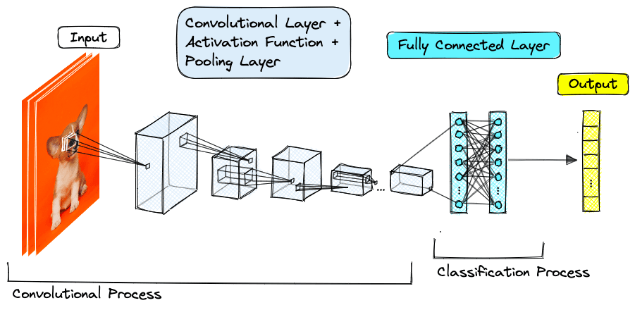
Typical architecture of a CNN.
CNNs use several convolutional layers stacked on top of one another. The first layers can recognize simple features, like edges, shapes, and textures. As the network gets deeper, it produces more “abstract” representations, eventually identifying concepts from mammals to dogs and even Siberian huskies.
Convolutional Neural Networks will be explained in more detail in the next chapter of Embedding Methods for Image Search.
These networks generally work best with many layers and large amounts of data, so they were overlooked. Shallow implementations lacked benefits over other networks, and deeper implementations were computationally unrealistic; the odds were stacked against these networks.
Despite these potential challenges, the authors of AlexNet won ILSVRC by a 9.8 percentage point margin with one of these models. It turns out they were the right people in the right place at the right time.
Several pieces came together for this to work. ImageNet provided the massive amounts of data required to train a deep CNN. A few years earlier, Nvidia had released CUDA, an API that enabled software access to highly-parallel GPU processing [12][13]. GPU power had reached a point where training AlexNet’s 60 million parameters became practical with the use of multiple GPUs.
AlexNet
AlexNet was by no means small. To make it work, the authors had to solve many problems. The model consisted of eight layers: five convolutional layers followed by three fully-connected linear layers. To produce the 1000-label classification needed for ImageNet, the final layer used a 1000-node softmax, creating a probability distribution over the 1000 classes.
![Network architecture of AlexNet [1].](https://www.pinecone.io/_next/image/?url=https%3A%2F%2Fcdn.sanity.io%2Fimages%2Fvr8gru94%2Fproduction%2F511d51bd1d1ec3b7155250bf7e53cfa6cb52f215-1339x503.png&w=3840&q=75)
Network architecture of AlexNet [1].
A key conclusion from AlexNet was that the depth of the network had been instrumental to its performance. That depth produced a lot of parameters, making training either impractically slow or simply impossible; if training on CPU. By training on GPU, training time could become practical. Still, high-end GPUs of the time were limited to ~3GB of memory, not enough to train AlexNet.
To make this work, AlexNet was distributed across two GPUs. Each GPU handled one-half of AlexNet. The two halves would communicate in specific layers to ensure they were not training two separate models.
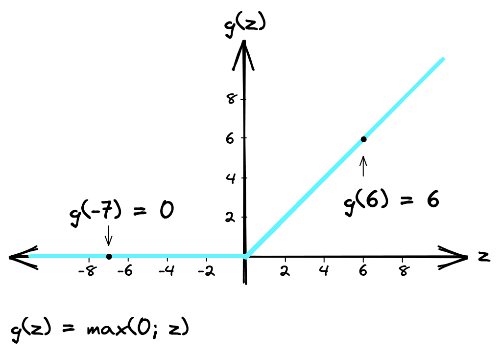
ReLU activation function.
Training time was reduced further by swapping the standard sigmoid or tanh activation functions of the time for Rectified Linear Unit (ReLU) activation functions.
![Results from a four-layer CNN with ReLU activation functions reached a 25% error rate on the CIFAR-10 dataset six times faster than the equivalent with Tanh activation functions [1].](https://www.pinecone.io/_next/image/?url=https%3A%2F%2Fcdn.sanity.io%2Fimages%2Fvr8gru94%2Fproduction%2F71282d56d034a67fd907516329544fecc6221abc-503x396.png&w=1080&q=75)
Results from a four-layer CNN with ReLU activation functions reached a 25% error rate on the CIFAR-10 dataset six times faster than the equivalent with Tanh activation functions [1].
ReLU is a simpler operation and does not require normalization like other functions to avoid activations congregating towards min/max values (saturation). Nonetheless, another type of normalization called Local Response Normalization (LRN) was included. Adding LRN reduced top-1 and top-5 error rates by 1.4% and 1.2% respectively [1].
Another critical component of AlexNet was the use of overlapping pooling. Pooling was already used by CNNs to summarize a group of activations in one layer to a single activation in the following layer.
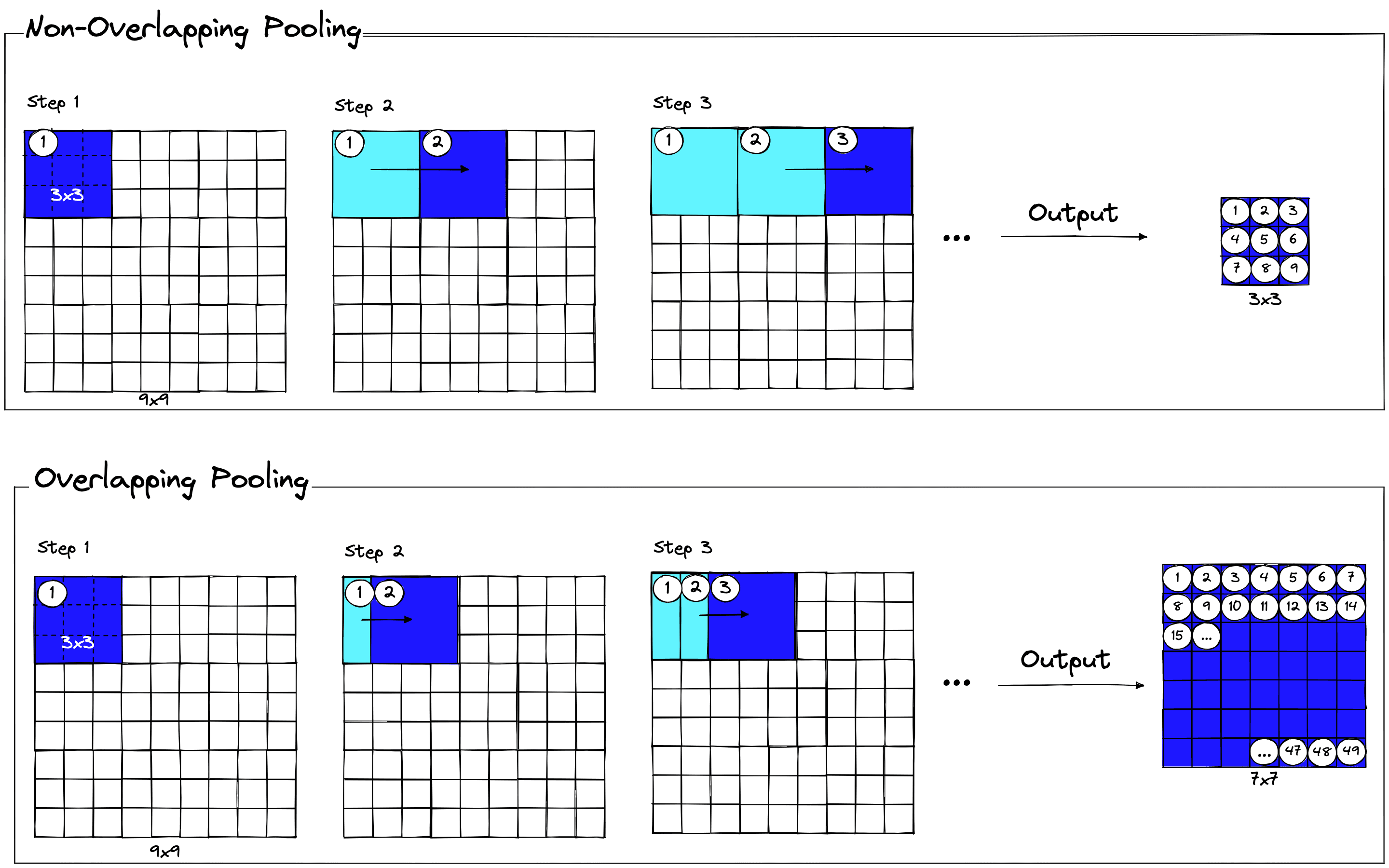
Overlapping pooling performs the same operation, but, as the pooling window moves across the preceding layer, it overlaps with the previous window. AlexNet found this to improve top-1 and top-5 error rates by 0.4% and 0.3%, respectively, and reduce overfitting.
AlexNet in Action
While it’s great to talk about all of this, it’s even better to see it implemented in code. You can find the Colab notebook here, TK, if you’d like to follow along.
Data Preprocessing
Let’s start by downloading and preprocessing our dataset. We will use a small sample from ImageNet hosted on HuggingFace.
In[2]:
# import dataset from HuggingFace
from datasets import load_dataset

imagenet = load_dataset(
    'Maysee/tiny-imagenet',
    split='valid',
    ignore_verifications=True  # set to True if seeing splits Error
)
imagenet
Out[2]:
Dataset({
    features: ['image', 'label'],
    num_rows: 10000
})
In[3]:
imagenet[0] # single recordOut[3]:
{'image': <PIL.JpegImagePlugin.JpegImageFile image mode=RGB size=64x64 at 0x105A9FA30>,
 'label': 0}
In[4]:
# check image type
type(imagenet[0]['image'])
Out[4]:
PIL.JpegImagePlugin.JpegImageFileIn[5]:
# view PIL images like so (in notebooks):
imagenet[0]['image']
Out[5]:
<PIL.JpegImagePlugin.JpegImageFile image mode=RGB size=64x64 at 0x165C59E20>The Maysee/tiny-imagenet dataset contains 100K and 10K labeled images in the train and validation sets, respectively. All images are stored as Python PIL objects. Preprocessing of these images consists of several steps:
- Convert all images to RGB format.
- Resize to fit AlexNet’s expected input dimensions.
- Convert to tensor format.
- Normalize values.
- Stack this set of tensors into a single batch.
We start with RGB; AlexNet assumes all images will have three color channels (Red, Green, and Blue). But many other formats are supported by PIL, such as L (grayscale), RGBA, and CMYK. We must convert any non-RGB PIL objects into RGB format.
In[5]:
# check for RGB, this image is okay
imagenet[0]['image'].mode
In[6]:
# 'L' is grayscale, and must be converted to RGB
imagenet[201]['image'].mode
In[7]:
imagenet[201]['image'] # we can see it is grayscaleOut[7]:
<PIL.JpegImagePlugin.JpegImageFile image mode=L size=64x64 at 0x15F634D30>In[8]:
img = imagenet[201]['image'].convert('RGB')
img  # it will still be shown as grayscale
Out[8]:
<PIL.Image.Image image mode=RGB size=64x64 at 0x15F634D60>AlexNet, and many other pretrained models, expect input images to be tensors of dimensions (3 x H x W), where 3 represents the three color channels. H and W are expected to have a dimensionality of at least 224 [14]. We must resize our images; this is done easily using torchvision.transforms.
In[9]:
from torchvision import transforms

# resize and crop to 224x224
preprocess = transforms.Compose([
    transforms.Resize(256),
    transforms.CenterCrop(224)
])

new_img = preprocess(imagenet[0]['image'])
new_img
Out[9]:
<PIL.Image.Image image mode=RGB size=224x224 at 0x176F5F130>Finally, we must normalize the image tensors to a range of [0, 1] using mean = [0.485, 0.456, 0.406] and std = [0.229, 0.224, 0.225] as per the implementation notes on PyTorch docs [14].
# resize and crop to 224x224
preprocess = transforms.Compose([
    transforms.ToTensor(),  # convert from PIL image to tensor before norm to avoid error
    transforms.Normalize(mean=[0.485, 0.456, 0.406], std=[0.229, 0.224, 0.225])
])

# final result is normalized tensor of shape (3, 224, 224)
new_img = preprocess(new_img)
We can combine all of this into a batch of 50 images. Rather than running preprocessing on our entire dataset and keeping everything in memory, we must process it in batches. For this example, we will only test the first 50 images as we know these should all be labeled as “goldfish”.
In[11]:
from tqdm.auto import tqdm
import torch

# define preprocessing pipeline
preprocess = transforms.Compose([
    transforms.Resize(256),
    transforms.CenterCrop(224),
    transforms.ToTensor(),
    transforms.Normalize(mean=[0.485, 0.456, 0.406], std=[0.229, 0.224, 0.225]),
])

inputs = []

for image in tqdm(imagenet[:50]['image']):
    # convert from grayscale to RBG
    if image.mode != 'RGB':
        image = image.convert("RGB")
    # prepocessing
    input_tensor = preprocess(image)
    inputs.append(input_tensor)

# convert batch list to tensor (as expected by the model)
inputs = torch.stack(inputs)
inputs.size()
Out[11]:
0%| | 0/50 [00:00<?, ?it/s]Out[11]:
torch.Size([50, 3, 224, 224])We have preprocessed our first batch and produced tensors containing 50 input tensors of shape (3, 224, 244), ready for inference with AlexNet.
Inference
To perform inference (e.g., make predictions) with AlexNet, we first need to download the model. We will download the pretrained AlexNet hosted by PyTorch.
In[12]:
import torch

# load pretrained alexnet from pytorch hub
model = torch.hub.load('pytorch/vision:v0.10.0', 'alexnet', pretrained=True)
model.eval()  # set model to evaluation mode (for inference)
Out[12]:
AlexNet(
  (features): Sequential(
    (0): Conv2d(3, 64, kernel_size=(11, 11), stride=(4, 4), padding=(2, 2))
    (1): ReLU(inplace=True)
    (2): MaxPool2d(kernel_size=3, stride=2, padding=0, dilation=1, ceil_mode=False)
    (3): Conv2d(64, 192, kernel_size=(5, 5), stride=(1, 1), padding=(2, 2))
    (4): ReLU(inplace=True)
    (5): MaxPool2d(kernel_size=3, stride=2, padding=0, dilation=1, ceil_mode=False)
    (6): Conv2d(192, 384, kernel_size=(3, 3), stride=(1, 1), padding=(1, 1))
    (7): ReLU(inplace=True)
    (8): Conv2d(384, 256, kernel_size=(3, 3), stride=(1, 1), padding=(1, 1))
    (9): ReLU(inplace=True)
    (10): Conv2d(256, 256, kernel_size=(3, 3), stride=(1, 1), padding=(1, 1))
    (11): ReLU(inplace=True)
    (12): MaxPool2d(kernel_size=3, stride=2, padding=0, dilation=1, ceil_mode=False)
  )
  (avgpool): AdaptiveAvgPool2d(output_size=(6, 6))
  (classifier): Sequential(
    (0): Dropout(p=0.5, inplace=False)
    (1): Linear(in_features=9216, out_features=4096, bias=True)
    (2): ReLU(inplace=True)
    (3): Dropout(p=0.5, inplace=False)
    (4): Linear(in_features=4096, out_features=4096, bias=True)
    (5): ReLU(inplace=True)
    (6): Linear(in_features=4096, out_features=1000, bias=True)
  )
)
We can see the network architecture of AlexNet here with five convolutional layers followed by three feed-forward linear layers. This represented a more efficient modification of the original AlexNet and was proposed by Krizhevsky in a later paper [15].
By default, the model is loaded to the CPU. We can run it here, but running on a CUDA-enabled GPU or MPS on Apple Silicon is more efficient. We do this by setting the device like so:
# move to device if available
device = torch.device(
    'cuda' if torch.cuda.is_available() else (
        'mps' if torch.backends.mps.is_available() else 'cpu'
    )
)
From this, we must always move the input tensors and model to the device before performing inference. Once moved, we run inference with model(inputs).
In[13]:
# move inputs and model to device
inputs = inputs.to(device)
model.to(device)

# run the model
with torch.no_grad():
    output = model(inputs).detach()
print(output.shape)
output
Out[13]:
tensor([[ 7.2008, 14.0141, -0.4883,  ...,  5.5724,  1.0935, -5.2350],
        [ 3.2615,  9.6214,  1.8129,  ..., -1.4830,  0.0919, -1.8151],
        [ 6.8251, 15.3777,  1.0032,  ...,  2.2704,  0.9593, -3.7721],
        ...,
        [ 3.5202, 10.5097, -3.0180,  ...,  2.2333,  0.5606, -2.0211],
        [ 3.6958, 13.0405,  0.9107,  ..., -1.4827,  2.8325, -5.1292],
        [ 3.4574,  8.3314, -2.0551,  ...,  1.7834,  1.5504, -3.1021]],
       device='mps:0')
In[15]:
# prediction
preds = torch.argmax(output, dim=1).cpu().numpy()
print(preds.shape)
preds
Out[15]:
array([  1,   1,   1,   1, 392,   1, 392,   1, 392,   1,   1,   1, 782,
         1, 392,  73, 392,   1,  29, 750, 392,  73, 738,   1,   1,   1,
         1, 491,   1,   1,   1,  98,   1,   1,   1,   1,   1,   1,   1,
         1,   1,   1,   1,   1,   1,   1,   1,   1,   1,   1])
The model will output a set of logits (output activations) for each possible class. There are 1000 of these for every image we feed into the model. The highest activation represents the class that the model predicts for each image. We convert these logits into class predictions with an argmax function.
Most of the predicted values belong to class 1. That has no meaning for us, so we cross check this with the PyTorch AlexNet classes like so:
In[17]:
import requests

res = requests.get("https://raw.githubusercontent.com/pytorch/hub/master/imagenet_classes.txt")
In[18]:
pred_labels = res.text.split('\n')
print(f"{len(pred_labels)}\n{pred_labels[1]}")
Clearly, the AlexNet model is predicting goldfish correctly. We can calculate the accuracy with:
sum(preds == 1) / len(preds)This returns an accuracy of 72% for the goldfish class. A top-1 error rate of 28% beats the reported average error rate of 37.5% from the original AlexNet paper. However, this is only for a single class, and the model performance varies from class to class.
That’s our overview of one of the most significant events in computer vision and machine learning. The ImageNet Challenge was hosted annually until 2017. By then, 29 of 38 contestants had an error rate of less than 5% [16], demonstrating the massive progress made in computer vision during ImageNet’s active years.
AlexNet was superseded by even more powerful CNNs. Microsoft Research Asia dethroned AlexNet as the winner of ILSVRC in 2015 [17]. Since then, many more CNN architectures have come and gone. Recently, the use of another network architecture known as a transformer has begun to disrupt CNNs domination of computer vision.
The final paragraph of the AlexNet paper proved almost prophetical for the future of AI and computer vision. They noted that they:
"did not use any unsupervised pre-training even though we expect it will help", and "our results have improved as we have made our network larger... we still have many orders of magnitude to go in order to match the infero-temporal pathway of the human visual system"
Unsupervised pre-training and ever larger models would later become the hallmark of ever better models.
Resources
[1] A. Krizhevsky, I. Sutskever, G. Hinton, ImageNet Classification with Deep Convolutional Neural Networks (2012), NeurIPS
[2] ImageNet Large Scale Visual Recognition Challenge (ILSVRC), ImageNet
[3] J. Dean, Machine Learning for Systems and Systems for Machine Learning (2017), NeurIPS 2017
[4] F. Li, Visual Recognition: Computational Models and Human Psychophysics (2005), Caltech
[5] G. Miller, R. Beckwith, C. Felbaum, D. Gross, K. Miller, Introduction to WordNet: An On-line Lexical Database (1993)
[6] D. Gershgorn, The data that transformed AI research — and possibly the world (2017), Quartz
[7] J. Deng, W. Dong, R. Socher, L. Li, K. Li, L. Fei-Fei, ImageNet: A large-scale hierarchical image database (2009), CVPR
[8] L. Ahn, L. Dabbish, Labeling images with a computer game (2004), Proc. SIGCHI
[9] I. Weber, S. Robertson, M. Vojnovic, Rethinking the ESP Game (2009), ACM
[10] A. Saini, Solving the web’s image problem (2008), BBC News
[11] O. Russakovsky, J. Deng, et. al., ImageNet Large Scale Visual Recognition Challenge (2015), IJCV
[12] F. Abi-Chahla, Nvidia’s CUDA: The End of the CPU? (2008), Tom’s Hardware
[13] A. Krizhevsky, cuda-convnet (2011), Google Code Archive
[14] AlexNet Implementation in PyTorch, PyTorch Resources
[15] A. Krizhevsky, One weird trick for parallelizing convolutional neural networks (2014)
[16] ILSVRC2017 Results (2017)
[17] K. He, X. Zhang, S. Ren, J. Sun, Deep Residual Learning for Image Recognition (2015)
Was this article helpful?