











This post is from 2023 and explains why a great algorithm like HNSW is not enough on its own to build a production vector database. Pinecone has never used HNSW: it has always run its own indexing, which today is per-slab adaptive indexing (Ananas, PQFS, and IVF) on serverless. → How Pinecone Works
The demand for vector databases has been rising steadily as workflows such as Retrieval Augmented Generation (RAG) have become integral to GenAI applications.
In response, many databases are now rushing to support vector search by integrating a vector index into their core offering. A common strategy they use is taking a well known vector-indexing algorithm, bolting it onto an existing (not vector-native) architecture, and calling it a day.
While this approach offers some convenience, it also has a fatal flaw: bolted-on vector indexes are inherently unable to handle the memory, compute, and scale requirements that real-world AI applications demand.
When we created Pinecone, we intentionally designed it around three tenets that would guarantee it meets and exceeds expectations for these types of real-world AI workloads:
We believe that these tenets are non-negotiable, and that bolt-on solutions that incorporate sidecar indexes into their core offerings are unable to satisfy them.
Part of the reason bolt-on vector databases are unable to meet these requirements is that most simply integrate a great vector-indexing algorithm, such as HNSW, and believe that that will translate to a great vector database.
But building a great vector database requires more than incorporating a great algorithm.
Below we’ll explain why even a great algorithm such as HNSW is not enough. Then we’ll take a look at one of Pinecone’s purpose-built indexing algorithms that runs on top of purpose-built architecture, and the difference it makes.
HNSW is a highly performant indexing algorithm that nets users great recall at high throughput. It’s used extensively throughout the vector-search world as the core of many notable open-source indexing libraries, such as NMSLIB and Faiss.
Like many graph-based algorithms, HNSW is fast. It gets its speed from its layered, hierarchical, graph structure, which allows it to quickly hone in on target neighborhoods (i.e. the potential matches for a user’s query).
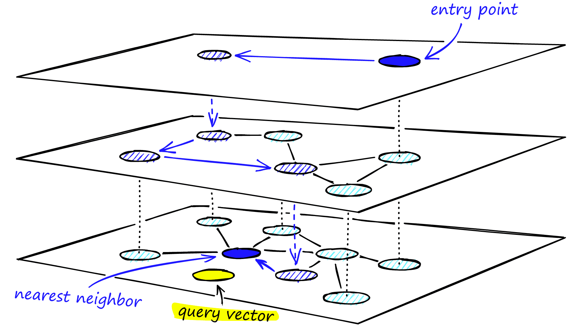
The search process through the multi-layered structure of an HNSW graph.
HNSW also generally gets accurate results (or “recall”). Its nodes and edges (i.e. the parts that make up the graph) connect semantically similar content, making it easy to find the most relevant vectors to a user’s query once within a target neighborhood.
Since each layer of the graph in an HNSW index is a subsample of the layer above, every time the algorithm travels down a layer, the search space (the universe of possible ‘right’ answers) gets reduced. This translates to ✅ speed and ✅ accuracy.
HNSW was designed for relatively static datasets, though, and production applications are anything but static. As your data changes, so do the vector embeddings that represent your data, and, consequently, so must the vector index. When you make frequent changes to a bolted-on HNSW index, its memory consumption begins to grow… a lot.
To deal with the growing memory consumption common CRUD operations like updates and deletes incur in HNSW indexes, you would have to do some or all of following:
It turns out the apparent convenience and initial performance of a bolted-on index comes with a significant cost and operational burden.
Exactly how bolted-on HNSW indexes balloon memory may be counter-intuitive, so let’s look at some of the reasons for this.
To understand the performance concerns that arise with HNSW indexes in a production environment, one has to understand how data’s size and makeup can affect memory consumption. In cloud computing, memory and compute are fundamentally coupled. Put (very) simply, this means that memory comes at the price of compute.
A large index takes up more space in memory. Since compute power is a function of available memory (and vice versa), if your data takes up lots of memory, you’ll need lots of compute to search over it and perform calculations.
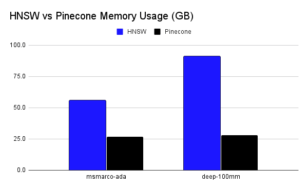
HNSW (default settings, optimized for memory) vs Pinecone (p2) memory usage. Tests conducted using two popular datasets: msmarco-ada and deep-100mm. Msmarco-ada contains 8.4M vectors of 1536 dimensions, while deep-100mm contains 100M vectors of 96 dimensions.
Above, you can see just how much more memory vectors stored in an HNSW index take up vs how much memory those same vectors take up when stored in a comparable graph-based Pinecone index (more on that later).
When your data is large but relatively static (e.g. census data), its “memory footprint,” and the compute required to search over it, is generally predictable and stable.
When your data is both large and dynamic (e.g. stock market data), however, managing the tradeoffs between memory and compute can get complicated. Each time a datapoint changes, its memory footprint also changes. And each time memory changes, the amount of compute needed changes, too.
One way you can mitigate memory issues is by tuning HNSW’s parameters: ef, k, M, efConstruction, and L:
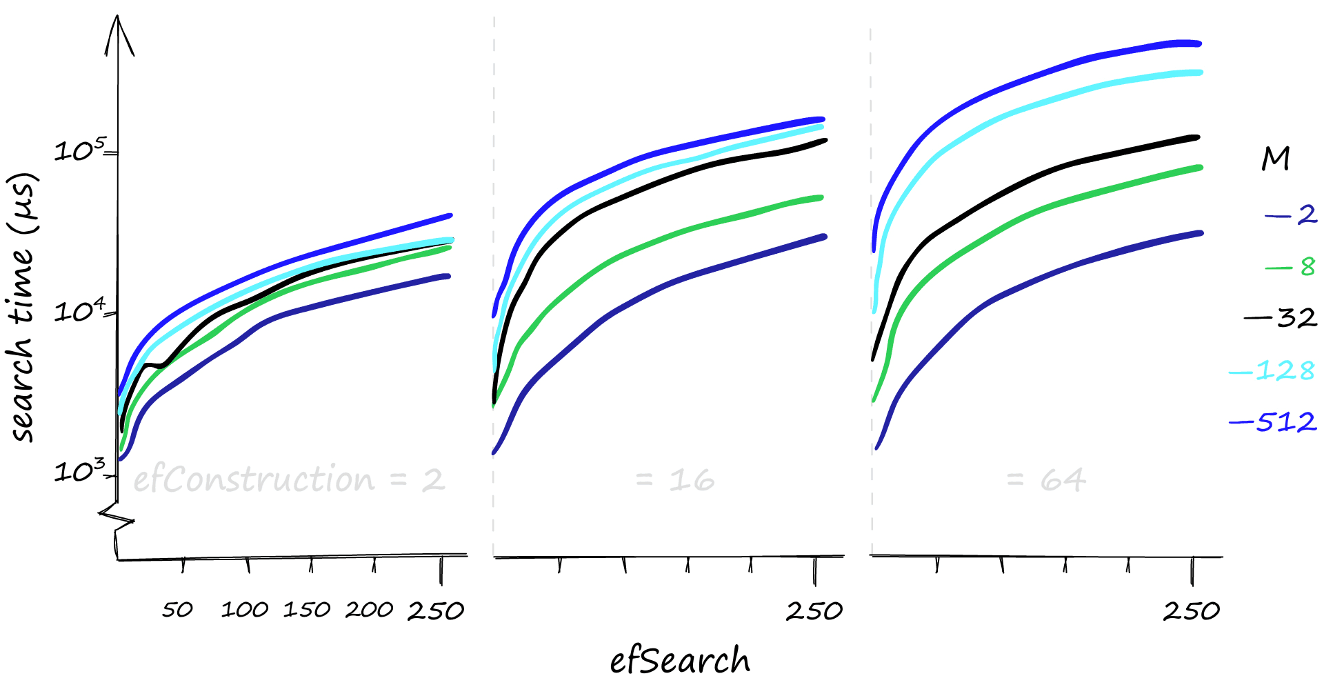
Search time in µs for various M, efConstruction, and efSearch parameters when searching for 1000 queries. Note that the y-axis is using a log scale.
On the graphs above, you can see the highly variable impact different values for these parameters can have on search time. By nature, these parameters need tuning anytime the data in the index changes – the perfect weightings on Monday might be vastly different from the perfect weightings on Tuesday, after a reindex.
To get a deeper understanding of how nutty things can get when dealing with memory, we’ll examine how an algorithm like HNSW handles a common CRUD operation: deletes.
Most, if not all, databases have the concepts of “hard” and “soft” deletes. Hard deletes are where you permanently delete data, whereas soft deletes are where one simply flags data as ‘to-be-deleted’ and deletes it at some later date. The common issue with soft deletes is that the to-be-deleted data has to live somewhere until it’s permanently removed. This means that even if you mark a record for deletion, it still takes up space in memory.
In non-vector databases, deleting data is as simple as removing the column, table, and/or row. In vector databases, specifically those powered by HNSW (or other layered graph algorithms), however, you have to rebuild the entire index from the ground up.
Since vector operations are so memory-intensive, this means that the memory space taken up by deleted data needs to be reclaimed immediately in order to maintain performance. This is where things get hard.
An inherent detail in layered graph indexes like those built by HNSW is that these graphs are sparse. This means that some layers have very few nodes (vectors). You can imagine, then, that if you delete a 1-node layer, all the subsequent layers that were attached to that 1-node layer get disconnected from the graph and are now in limbo. These disconnections break the index.
To fix the graph (repair the connections), you must rebuild the index entirely from scratch. Even if you want to add or update vectors, you must first delete an old vector. Every change requires a delete.
To avoid doing this for every single change, vector indexes mark to-be-deleted data with something called a tombstone. This process is a type of soft delete. At retrieval time, this tombstone acts as a flag to the system, indicating that the piece of data is not eligible to be returned to the user.
Eventually, though, this to-be-deleted data has to be permanently removed from the graph, breaking the graph.
In order to do a “hard delete” and permanently remove data to a sparse graph index like the one made by HNSW, the index has to be rebuilt.
This might not seem like a big deal at first. But if your index is being completely rebuilt periodically, how can it also always be accessible to users? Well, it can’t.
You can mitigate this unavailability by creating a static copy of the index to direct user traffic to during reindexing (blue-green deployment). This means that users are getting served stale data (plus, the storage requirements might be huge to replicate a whole index). This can be make or break if your business relies on surfacing real-time or nearly-real-time data.
For a production-grade vector database, consistent data availability and fresh data are necessities.
Inefficient memory (and therefore cost), the need for expert parameter tuning, data unavailability, and data staleness are some of the reasons we at Pinecone don’t think that a great algorithm like HNSW makes a great foundation for a vector database.
Great, purpose-built vector databases need more than great algorithms.
Returning to our design requirements, great vector databases must be:
Easy to use and operate —Your database should “just work”
As a SaaS company, we want to give you the freedom to concentrate on what matters: building the product.
Since vector databases are a core piece of infrastructure within GenAI applications, they should just work. Simple as that. There should be no need for you to spend endless hours tuning complex algorithms or adding error handling to check that an index can handle simple CRUD operations.
Users of GenAI applications powered by Pinecone should be confident that they’re getting the freshest, most relevant data possible. Developers of GenAI applications powered by Pinecone should be confident that the infrastructure will manage itself and the serving cost will be predictable and affordable.
Flexible — Your database should meet multiple user needs.
Products that rely on vector databases have a variety of priorities. With Pinecone, developers can choose different index types, based on the performance characteristics they value most. Each of Pinecone’s index types is powered by a bespoke algorithm designed to deliver towards a particular use case.
Performant and cost-effective at any scale — Your database should manage memory, and therefore cost, efficiently at any scale.
The scale and makeup of your data should not impact your database’s performance. Under the hood, Pinecone is powered by vector-optimized data structures and algorithms to ensure your indexes stay up and running, always.
At Pinecone, there are two families of indexes: the p-family and the s-family. These families were designed intentionally with an eye towards meeting different user needs and avoiding memory problems, thereby maximizing cost efficiency.
P-family
The p-family of indexes is optimized for memory. There are two offerings in this family: our p1 and p2 indexes. These indexes are both stored in-memory and are highly efficient. They can either guarantee extremely fast data updates (data freshness) and moderate throughput (p1), or less-fast data updates and high throughput (p2).
S-family
The s-family of index types is optimized for storage. In this index type, the vectors themselves are stored and fetched from local SSD. This allows us to take advantage of the cost mechanics between RAM and SSD. There is currently one offering in this family: our s1 index.
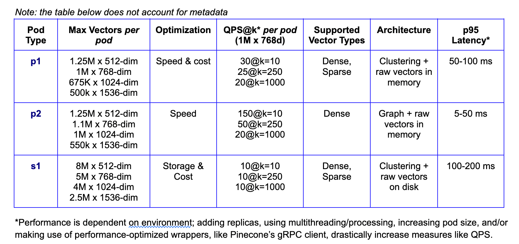
Table showing the differences between Pinecone’s three index types.
Each index type has different strengths, as seen above. If users want the best balance between speed and cost, they’d choose p1; if users care more about speed than cost, they’d choose p2; and if users care most about storage (e.g. low throughput use cases), they’d choose s1.
To illustrate the intentionality and thought we have put into the design of each of our index types, we’ll take a deep dive into the custom algorithm that powers our p2 indexes. We’ll situate its performance within our earlier conversation about HNSW and the larger theme of bolt-on solutions vs purpose-built vector databases.
In order to build an index type that would empower us at Pinecone to meet the three tenets we believe make a great vector database (easy to use, flexible, and performant at any scale), we took the road less traveled and developed our own algorithm.
The Pinecone Graph Algorithm, or PGA, is similar to HNSW in that it also builds a graph structure. Graphs are fast, and we like fast. But that is where its similarities end.
PGA is based off of Microsoft’s Vamana (commonly referred to as FreshDiskANN) algorithm. Unlike HNSW, which builds a hierarchical graph structure (sparse graph), FreshDiskANN builds a flat-graph structure (dense graph).
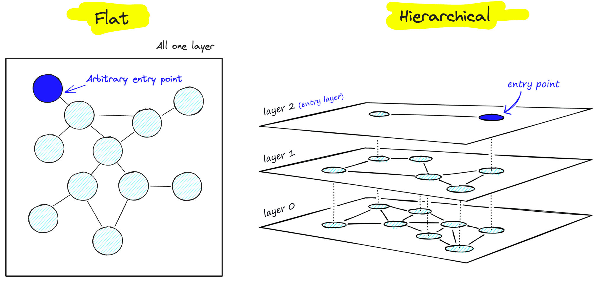
Flat graph structure (e.g. FreshDiskANN) vs Hierarchical graph structure (e.g. HNSW).
FreshDiskANN uses a small, fast storage system (memory buffer) for new data points and a large, less-fast storage system (disk) for older data points. Once the memory buffer hits capacity, it merges its items into the index on disk, maintaining data freshness.
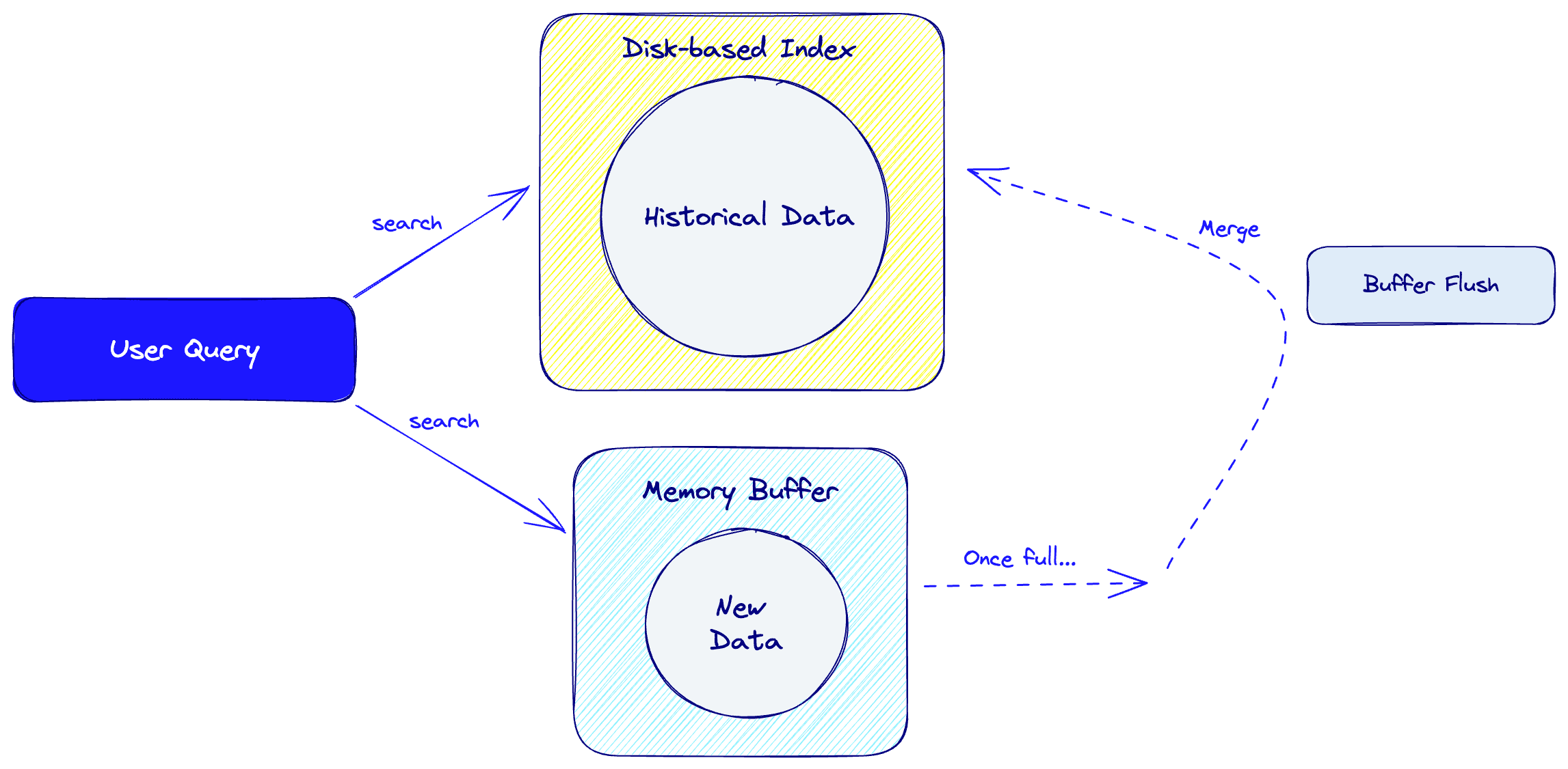
Diagram of FreshDiskANN algorithm.
When searching for retrieval candidates, the algorithm searches over both storage units, combining the results. It naturally performs periodic maintenance operations, such as compaction and splitting, which optimize the index. Its flat structure is also ideal for caching and parallel processing, which increase speed and recall.
Since we optimized our p2 indexes for throughput, however, we built PGA to keep all data in RAM, much like HSNW (and unlike FreshDiskANN). To avoid the memory bloat issues that usually come with keeping data in RAM, we then apply scalar quantization to the in-memory data.
In addition to PGA being memory efficient by nature (more on that below), Pinecone has various backpressure systems that keep memory consumption level.
Backpressure is a software design mechanism by which some downstream component(s) applies pressure ”back” to an upstream process in order to give itself time to catch up. For example, if a user is upserting data into a Pinecone index and a Kafka writer is getting overwhelmed, the writer can send a signal to the upstream process telling it to slow down for a little bit.
End users never see the impact of this process; it’s all handled behind the scenes. We keep track of memory usage and its limits via a “fullness” metric. Monitoring this fullness metric ensures users don’t run into out of memory (OOM) errors in production.
As you might recall from our earlier conversation, a problem with layered indexing algorithms is that CRUD operations like deletes require rebuilding the index from scratch. This results in downtime and stale data.
One of the advantages of working with a flat, graph-based data structure instead of a hierarchical, graph-based data structure is that flat graphs are dense. Their density makes it significantly harder to create “orphan nodes” when deleting/adding/updating data (i.e. breaking the graph).
With a dense graph, rebuilding the connections between neighbor nodes is incremental. While we still use common soft-delete strategies like tombstones until we hard-delete records later, this incrementality allows us to avoid rebuilding the index from scratch at all. Instead, we just have to rebuild parts of the graph locally.
Since we never have to completely rebuild the index, your index is always available to the end user.
Moreover, the density of the PGA graph (along with the locality of deletes/additions/updates) allows us to achieve O(sec) data freshness. This means that as soon as data is added or removed from the index, that new data is immediately available to the end user for querying.
The flat-graph structure, scalar quantization of the vectors, and our built-in backpressure mechanisms all contribute to stellar performance. PGA is both extremely fast and extremely good at retrieving relevant results (recall).
Below, there are two graphs that illustrate the PGA’s performance across two popular datasets for benchmarking vector algorithms: fashion-mnist-784-euclidean and sift-128-euclidean. PGA is represented by the brightest blue line at the top:
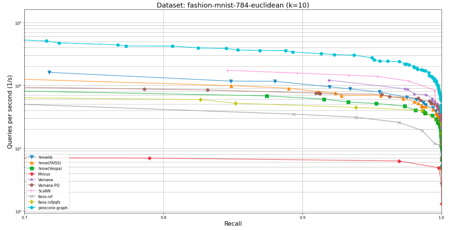

Testing was done in Oct 2022 on a GCP virtual machine with 8 vCPU and 32GB RAM, using 7 threads (vectors not quantized).
As you can see above, PGA outperforms not only HNSW and its variants, but also popular indexing algorithms across the board, such as Vamana itself, IVF, and ScaNN.
In summary, while developing an algorithm from scratch was a process few, if any, vector database providers undertake, the benefits we were able to pass onto developers was well worth the effort.
Overall, bolt-on solutions have inherent limitations when it comes to managing the memory and compute demands of today’s GenAI applications. Enabling a sidecar index that is based on an algorithm like HNSW is not a robust enough foundation for a production-level vector database.
Developers of GenAI applications today need a solution that is designed entirely with vectors in mind. This solution should be easy to use, flexible, performant, and cost effective. That’s what we built with Pinecone, and you can try it yourself for free.
We would love to hear your feedback. Reach out to us on Twitter and LinkedIn.
此内容由惯性聚合(RSS阅读器)自动聚合整理,仅供阅读参考。 原文来自 — 版权归原作者所有。