Convolutional Neural Networks (CNNs) have been the undisputed champions of Computer Vision (CV) for almost a decade. Their widespread adoption kickstarted the world of deep learning; without them, the field of AI would look very different today.

Before deep learning with CNNs, CV applications relied on brittle edge detection algorithms, color profiles, and a plethora of manually scripted processes. These could rarely be applied across different datasets or use cases.

The result is that every dataset and every use-case required significant manual intervention and domain-specific knowledge, rarely producing performance acceptable for broader use.

Deep-layered CNNs changed this. Rather than manual feature extraction, CNNs proved capable of doing this automatically for a vast number of datasets and use cases. All they needed was training data.

Big data with deep CNNs have remained the de-facto standard in computer vision. New models using vision transformers (ViT) and multi-modality may change this in the future, but for now CNNs still dominate state-of-the-art benchmarks in vision. In this hands-on article we will learn why.

What Makes a CNN?

CNNs are neural networks known for their performance on image datasets. They are characterized by something called a convolutional layer that can detect abstract features of an image. These images can be shifted, squashed, or rotated; if a human can still recognize the features, a CNN likely can too.

Because of their affinity to image-based applications, we find CNNs used for image classification, object detection, object recognition, and many more tasks within the realm of CV.

Deep-layered CNNs are any neural network that satisfies two conditions; (1) they have many layers (deep), and (2) they contain convolutional layers. Beyond that, networks can have many features, including pooling, normalization, and linear layers.

Convolutional Layers

An image is a big array of pixel activation values. These arrays are followed by more arrays of (initially random) values – the weights – that we call a “filter” or “kernel”. A convolutional layer is an element-wise multiplication between these pixel values and the filter weights – which are then summed.

This element-wise operation followed by the sum of the resulting values is often referred to as the “scalar product” because it results in a single scalar value [2].

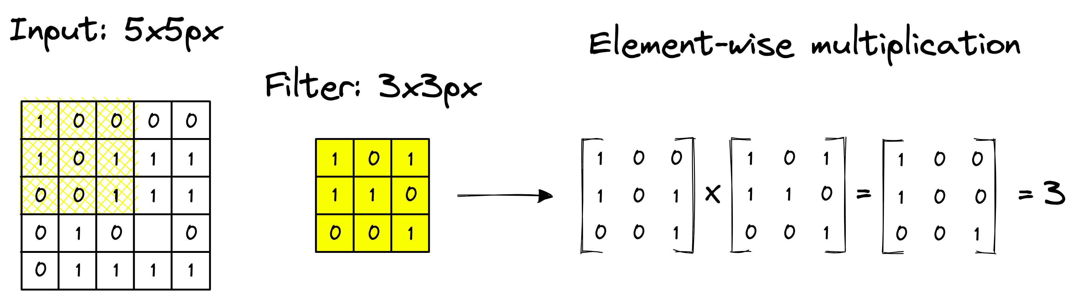
Considering the above example, when the 3x3 filter is applied to the input image starting from the top-left, the resulting value from the element-wise multiplication is 3.

We don’t return a single scalar value because we perform many of these operations on each layer. For each convolutional layer, the filter slides (or “convolves”) over the previous layer’s matrix (or image) from left-to-right and top-to-bottom.

The filter can detect specific local features such as edges, shapes, and textures by sliding over the image.

This convolution has a parallel in signal processing. Given an input audio wave , we “convolve” a filter  over it to produce a modified audio wave. See the appendix for a more detailed explanation.

The convolution output is called a “feature map” or “activation map” thanks to the representation or activations of detected features from the input layer.

As the element-wise multiplication of the filter outputs a single value after processing multiple input values, we need to be mindful of excessive information loss via dimensionality reduction (i.e., compression).

We may want to increase or decrease the amount of compression our filters create. Compression is controlled using the filter size and how quickly it moves across the image (the stride).

The stride defines the number of pixels a filter moves after every calculation. By increasing the stride, the filter will travel across the entire input image in fewer steps, outputting fewer values and producing a more compressed feature map.

There are some surprising effects of image compression, and one that we must be careful of is the filter’s interaction with the border areas of an input layer.

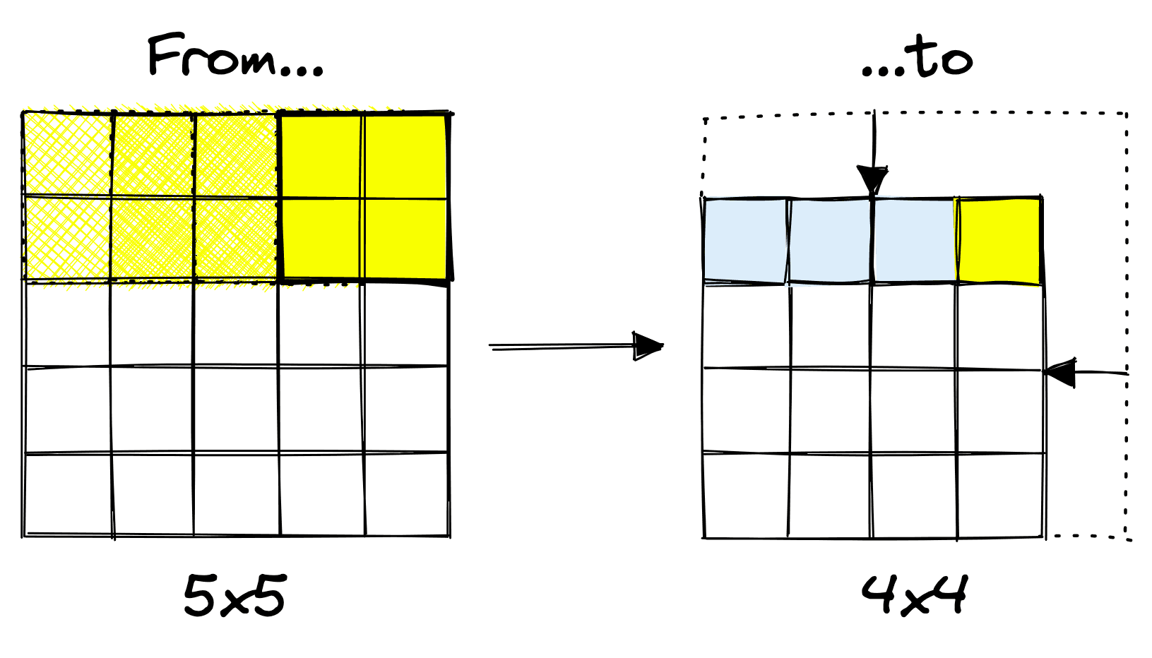
The border effects on small images can result in a rapid loss of information for images containing too little information. To avoid this, we either reduce compression using the previously discussed techniques (filter size and stride) or add padding.

Adding a set of zero-value pixels around the image allows us to limit or prevent compression between layers. In the example above, the operation without padding causes compression of 10x10 pixels into 8x8 pixels. With padding, no compression occurs (a 10x10 feature map is output). TK 10x10??

For larger images, compression is less likely to cause problems. However, when working with smaller images, padding acts as an easy and effective remedy to border effects,

Depth

We mentioned that deep-layered CNNs were what took CV to new heights. The AlexNet authors found the depth of networks to be a key component for higher performance [1]. Each successive layer extracts features from the previous layer (and previously extracted features). This chain of consecutive extractions produces ever more “abstract” features that can better represent images in more “human” terms.

A shallow network may recognize that an image contains an animal, but as we add another layer, it may identify a dog. Adding another may result in identifying specific breeds like Staffordshire Bull Terrier or Husky. More layers generally result in recognition of more abstract and specific concepts.

Activation Functions

Activation functions are a common feature in every type of neural network. They add non-linearity to networks, enabling the representation of more complex patterns.

In the past, CNNs often used hidden layer activation functions like sigmoid or tanh. However, in 2012 a new activation function called a Rectified Linear Unit was popularized through its use in AlexNet, the best-performing CNN of its time.

Nowadays, ReLU is still a popular choice. It is simpler than tanh and sigmoid and does not require normalization to avoid saturation (i.e., activations congregating towards the min/max values).

Pooling Layers

Output feature maps are highly sensitive to small changes in the location of input features [3]. To some degree, this can be useful, as it can tell us the difference between a cat’s face and a dog’s face. However, if an eye is two pixels further to the left than expected, the model should still be able to identify a face.

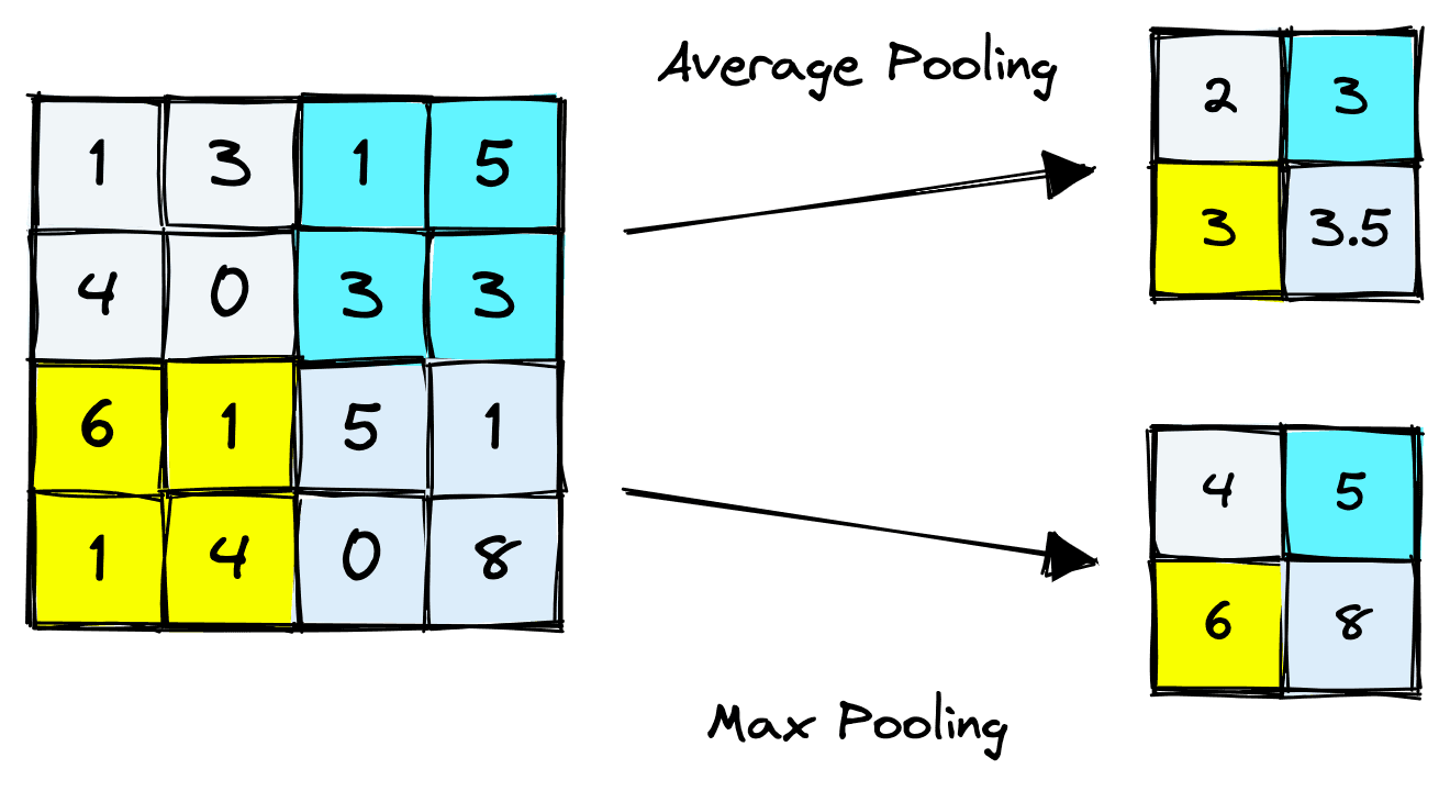
CNNs use pooling layers to handle this. Pooling layers are a downsampling method that compresses information from one layer into a smaller space in the next layer.

An effect of pooling is that information across several pixels is compressed into a single activation, essentially “smoothing out” variations across groups (or patches) of pixels.

The two most common pooling methods are average pooling and max pooling. Average pooling takes the average of activations in the window, whereas max pooling takes their maximum value.

Fully-Connected Layers

Fully connected linear layers are another common feature of CNNs. They are neural networks in their most stripped-down form; the dot product between inputs and layer weights with a bias term and activation function.

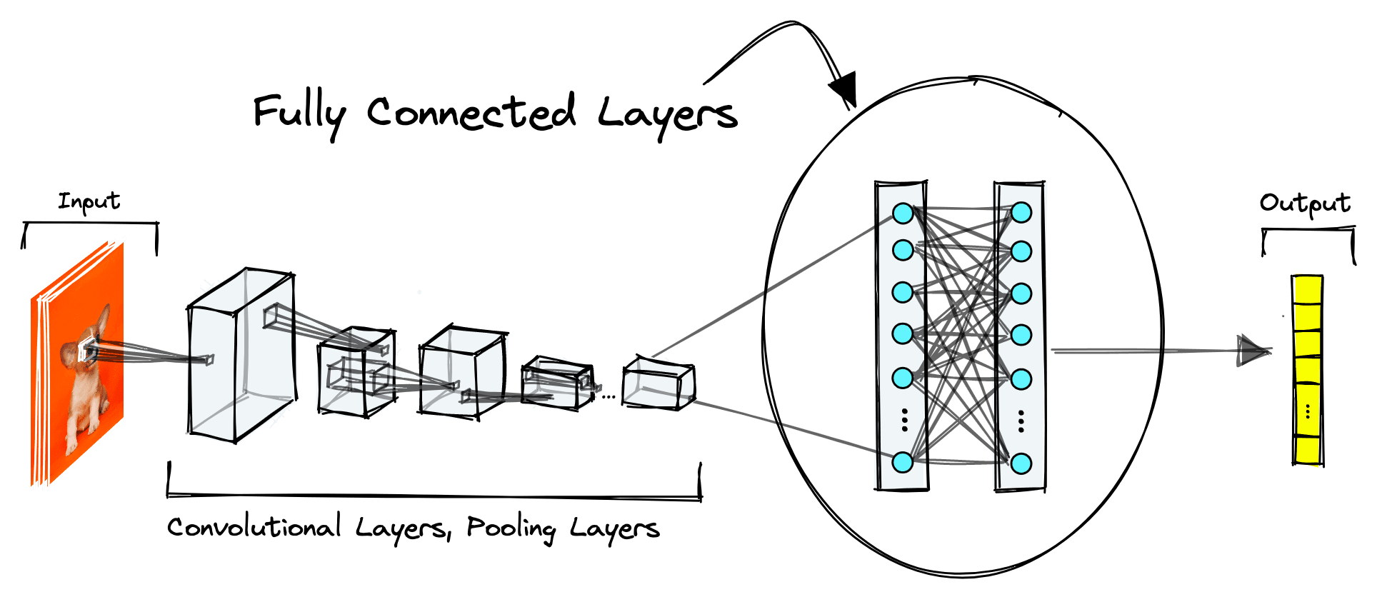
These layers are usually found towards the end of a CNN and handle the transformation of CNN embeddings from 3D tensors to more understandable outputs like class predictions.

Often within these final layers, we will find the most information-rich vector representations of the data being input to the model. In the next chapter of the ebook, we will explore these in more depth for use in content-based image retrieval (CBIR).

For now, let’s focus on the task of classification. Classifiers tend to apply a softmax activation function that creates a probability distribution across the final output nodes — where each node represents a specific class.

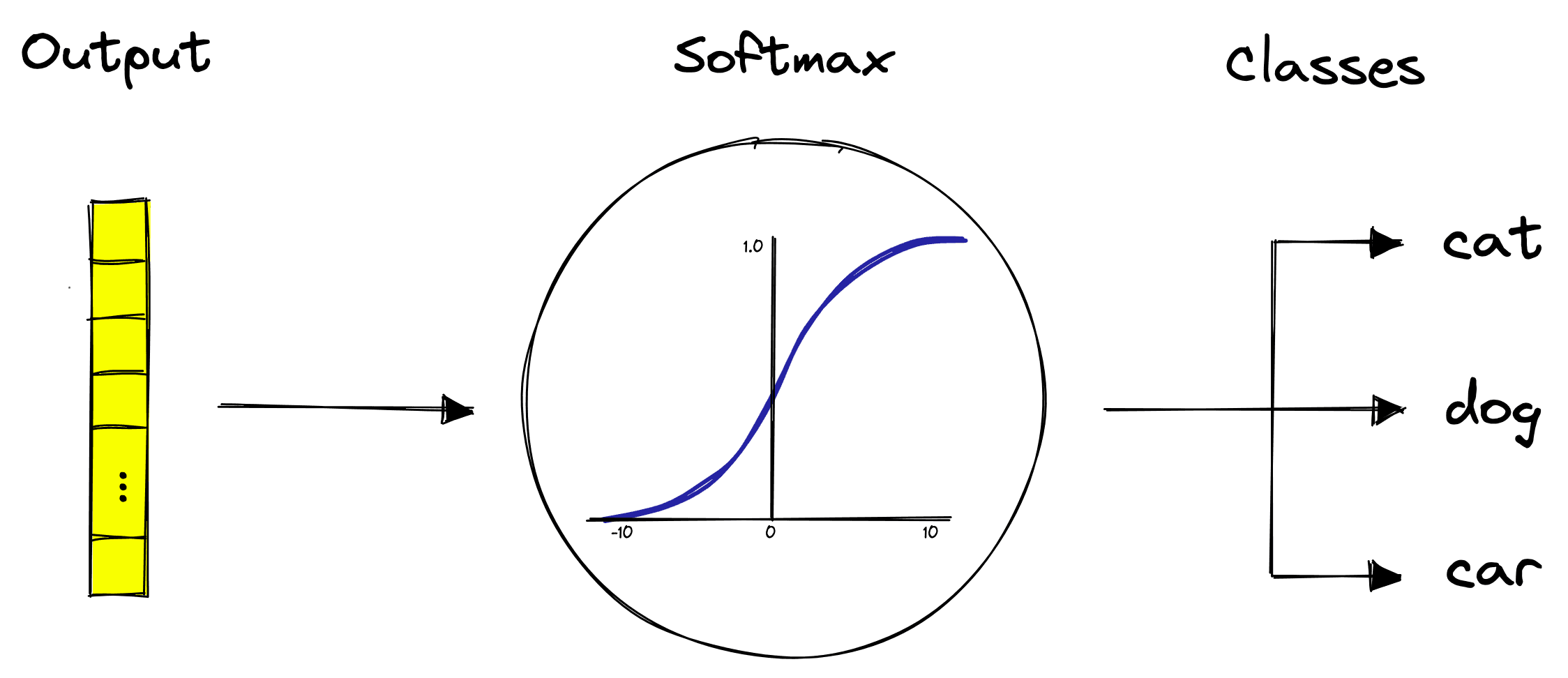
After these final fully-connected layers, we have our predictions.

These are a few of the most common components of CNNs, but with time many different types of CNNs with different network architectures were designed. So there is no “specific” architecture, just a set of guideposts in the form of high-performing networks.

Popular Architectures

Throughout the years, there have been several hugely successful CNN architectures. We will take a high-level look at a few of the most relevant.

LeNet

LeNet is the earliest example of a “deep” CNN, developed in 1998 by Yann LeCun, et. al. [4]. Many of us have likely interacted with LeNet as Bell Labs licensed it to banks around the globe for reading the digits on handwritten cheques.

This first example of a commercially successful deep CNN was surprisingly the only such example of a successful deep CNN for another 14 years.

AlexNet

October 2012 is widely regarded as ground zero for the birth of deep learning. The catalyst was AlexNet winning the ImageNet ILSVRC challenge [1]. AlexNet can be seen as a continuation of LeNet, using a similar architecture but adding more layers, training data, and safeguards against overfitting.

After AlexNet, the broader community of CV researchers began focusing on training deeper models with larger datasets. The following years saw variations of AlexNet continue winning ILSVRC and reaching ever more impressive performance.

VGGNet

AlexNet was dethroned as the winner of ILSVRC in 2014 with the introduction of VGGNet, developed at Oxford University [5]. Many variants of VGGNet were developed, characterized by the number of layers they contained, such as 16 total layers (13 convolutional) for VGGNet-16, and 19 total layers for VGGNet-19.

ResNet

ResNet became the new champion of CV in 2015 [6]. The ResNet variants were much deeper than before, the first containing 34 layers. Since then, 50+ layer ResNet models have been developed and hold state-of-the-art results on many benchmarks.

ResNet was inspired by VGGNet but added smaller filters and a less complex network architecture. Shortcut connections between different layers were also added, giving the name of Residual Network (ResNet).

Without these shortcuts, the greater depth of ResNet results in information loss over the many layers of transformations. Adding the shortcuts enabled information to be maintained across these greater distances.

Classification with CNNs

We’ve understood the standard components of CNNs and how these work together to extract abstract — but meaningful — features from images.

We also looked at a few of the most popular architectures. Let’s now put all of this together and work through an application of a CNN for image classification.

Data Preprocessing

As usual, our first task is data preparation and preprocessing. We will use a popular image classification dataset called CIFAR-10 hosted on Hugging Face datasets.

# import CIFAR-10 dataset from HuggingFace
from datasets import load_dataset

dataset_train = load_dataset(
    'cifar10',
    split='train', # training dataset
    ignore_verifications=True  # set to True if seeing splits Error
)

dataset_train

Dataset({
    features: ['img', 'label'],
    num_rows: 50000
})

# check how many labels/number of classes
num_classes = len(set(dataset_train['label']))
num_classes

# let's view the image (it's very small)
dataset_train[0]['img']

<PIL.PngImagePlugin.PngImageFile image mode=RGB size=32x32>

Here we have specified that we want the training split of the dataset with split='train'. We return 50K images split across ten classes from this.

Most CNNs can only accept images of a fixed size. To handle this, we will reshape all images to 32x32 pixels using torchvision.transforms; a pipeline built for image preprocessing.

import torchvision.transforms as transforms

# image size
img_size = 32

# preprocess variable, to be used ahead
preprocess = transforms.Compose([
    transforms.Resize((img_size,img_size)),
    transforms.ToTensor()
])

The preprocess pipeline handles the height and width of our images but not the depth. Every image has a number of “color channels” that define its depth. For RGB images, there are three color channels; red, green, and blue, whereas grayscale images have just one.

Datasets commonly contain images with different color profiles, so we must convert them into a set format. We will use RGB, and as our images are all Python PIL objects, the color format is stored in an attribute called mode. The mode will be RGB for RGB images and L for grayscale images.

We perform the conversion to RGB and also perform the preprocess transformations like so:

from tqdm.auto import tqdm

inputs_train = []

for record in tqdm(dataset_train):
    image = record['img']
    label = record['label']

    # convert from grayscale to RGB
    if image.mode == 'L':
        image = image.convert("RGB")
        
    # prepocessing
    input_tensor = preprocess(image)
    
    # append to batch list
    inputs_train.append([input_tensor, label]) 

  0%|          | 0/50000 [00:00<?, ?it/s]

print(len(inputs_train), inputs_train[0][0].shape)

50000 torch.Size([3, 32, 32])

Leaving us with 50,000 training examples, each a 3x32x32-dimensional tensor. The tensors are normalized to a [0,1][0,1] range by the transforms.ToTensor() step.

Right now, this normalization does not consider the pixel values of our overall set of images. Ideally, we should normalize by the mean and standard deviation values specific to this dataset. For this dataset, these are:

mean = [0.4670, 0.4735, 0.4662]
std = [0.2496, 0.2489, 0.2521]

This normalization step is applied by another transformers.Compose step like so:

preprocess = transforms.Compose([
    transforms.Normalize(mean=mean, std=std)
])

for i in tqdm(range(len(inputs_train))):
    # prepocessing
    input_tensor = preprocess(inputs_train[i][0])
    # replace with normalized tensor
    inputs_train[i][0] = input_tensor

We repeat the steps above for a test set that we will use for validating our CNN classifier performance. The validation set is also downloaded from Hugging Face datasets via load_dataset by switching the earlier split parameter to 'test':

dataset_val = load_dataset(
    'cifar10',
    split='test',  # test set (used as validation set)
    ignore_verifications=False  # set to True if seeing splits Error
)

The validation set must also be preprocessed, find the code for it here.

Both train and validation splits are added into DataLoader objects. The data loaders shuffle, batch, and load data into the model during training or inference (validation).

batch_size = 64

# add to dataloaders
dloader_train = torch.utils.data.DataLoader(
  	inputs_train,
    batch_size=batch_size,
    shuffle=True
)

dloader_val = torch.utils.data.DataLoader(
  	inputs_val,
    batch_size=batch_size,
    shuffle=False
)

With that, our data is ready, and we can move on to building and then training our CNN.

CNN Construction

We can start building our CNN by creating a ConvNeuralNet class that will contain all our network layers and define the order of transformations through the network. The network will look like this:

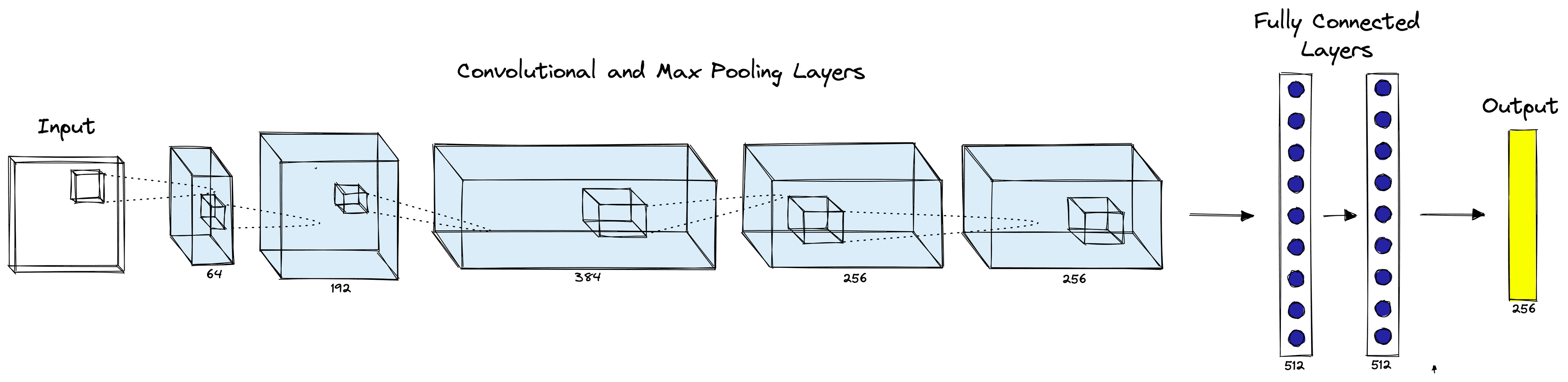
# creating a CNN class
class ConvNeuralNet(nn.Module):
	#  determine what layers and their order in CNN object 
    def __init__(self, num_classes):
        super(ConvNeuralNet, self).__init__()
        self.conv_layer1 = nn.Conv2d(in_channels=3, out_channels=64, kernel_size=4, padding=1)
        self.relu1 = nn.ReLU()
        self.max_pool1 = nn.MaxPool2d(kernel_size=3, stride=2)

        self.conv_layer2 = nn.Conv2d(in_channels=64, out_channels=192, kernel_size=4, padding=1)
        self.relu2 = nn.ReLU()
        self.max_pool2 = nn.MaxPool2d(kernel_size=3, stride=2)

        self.conv_layer3 = nn.Conv2d(in_channels=192, out_channels=384, kernel_size=3, padding=1)
        self.relu3 = nn.ReLU()
        
        self.conv_layer4 = nn.Conv2d(in_channels=384, out_channels=256, kernel_size=3, padding=1)
        self.relu4 = nn.ReLU()

        self.conv_layer5 = nn.Conv2d(in_channels=256, out_channels=256, kernel_size=3, padding=1)
        self.relu5 = nn.ReLU()
        self.max_pool5 = nn.MaxPool2d(kernel_size=3, stride=2)
        
        self.dropout6 = nn.Dropout(p=0.5)
        self.fc6 = nn.Linear(1024, 512)
        self.relu6 = nn.ReLU()
        self.dropout7 = nn.Dropout(p=0.5)
        self.fc7 = nn.Linear(512, 256)
        self.relu7 = nn.ReLU()
        self.fc8 = nn.Linear(256, num_classes)
    
    # progresses data across layers    
    def forward(self, x):
        out = self.conv_layer1(x)
        out = self.relu1(out)
        out = self.max_pool1(out)
        
        out = self.conv_layer2(out)
        out = self.relu2(out)
        out = self.max_pool2(out)

        out = self.conv_layer3(out)
        out = self.relu3(out)

        out = self.conv_layer4(out)
        out = self.relu4(out)

        out = self.conv_layer5(out)
        out = self.relu5(out)
        out = self.max_pool5(out)
        
        out = out.reshape(out.size(0), -1)
        
        out = self.dropout6(out)
        out = self.fc6(out)
        out = self.relu6(out)

        out = self.dropout7(out)
        out = self.fc7(out)
        out = self.relu7(out)

        out = self.fc8(out)  # final logits
        return out

After designing the network architecture, we initialize it — and if we have access to hardware acceleration (through CUDA or MPS), we move the model to that device.

import torch

device = "cuda" if torch.cuda.is_available() else "cpu"
# set the model to device
model = ConvNeuralNet(num_classes).to(device)

Next, we set the loss and optimizer functions used during training.

# set loss function
loss_func = nn.CrossEntropyLoss()
# set learning rate 
lr = 0.008
# set optimizer as SGD
optimizer = torch.optim.SGD(
    model.parameters(), lr=lr
) 

We will train the model for 50 epochs. To ensure we’re not overfitting to the training set, we pass the validation set through the model for inference only at the end of each epoch. If we see validation set performance suddenly degrade while train set performance improves, we are likely overfitting.

The training and validation loops are written like so:

num_epochs = 50
for epoch in range(num_epochs):
    model.train()
		# load in the data in batches
    for i, (images, labels) in enumerate(dloader_train):  
        # move tensors to the configured device
        images = images.to(device)
        labels = labels.to(device)
        
        # forward propagation
        outputs = model(images)
        loss = loss_func(outputs, labels)
        
        # backward propagation and optimize
        optimizer.zero_grad()
        loss.backward()
        optimizer.step()
        
    # at end of epoch check validation loss and acc
    with torch.no_grad():
      	# switch model to eval (not train) model
        model.eval()
        correct = 0
        total = 0
        all_val_loss = []
        for images, labels in dloader_val:
            images = images.to(device)
            labels = labels.to(device)
            outputs = model(images)
            total += labels.size(0)
            # calculate predictions
            predicted = torch.argmax(outputs, dim=1)
            # calculate actual values
            correct += (predicted == labels).sum().item()
            # calculate the loss
            all_val_loss.append(loss_func(outputs, labels).item())
        # calculate val-loss
        mean_val_loss = sum(all_val_loss) / len(all_val_loss)
        # calculate val-accuracy
        mean_val_acc = 100 * (correct / total)
    print(
        'Epoch [{}/{}], Loss: {:.4f}, Val-loss: {:.4f}, Val-acc: {:.1f}%'.format(
            epoch+1, num_epochs, loss.item(), mean_val_loss, mean_val_acc
        )
    )

After training for 50 epochs, we should reach a validation accuracy of ~80%. We can save the model to file and load it again with the following:

# save to file
torch.save(model, 'cnn.pt')
# load from file and switch to inference mode
model = torch.load('cnn.pt')
model.eval()

Inference

Now that we have a fine-tuned CNN model let’s look at how we can do image classification. We will use the same test set of CIFAR-10 for this step (ideally, we would not use the same data in our validation and test sets).

First, we preprocess the images using the same preprocess pipeline as before and stack every processed image tensor into a single tensor batch.

input_tensors = []
for image in dataset_test['img'][:10]:
    tensor = preprocess(image)
    input_tensors.append(tensor.to(device))

# we have 10 tensors
len(input_tensors)

# all 32x32 dimensional with 3 color channels
input_tensors[0].shape

# stack into a single tensor
input_tensors = torch.stack(input_tensors)
input_tensors.shape

torch.Size([10, 3, 32, 32])

We process the tensors through the model and use an argmax function to retrieve the predictions. The predictions are all integer values, so we retrieve the textual names within the dataset features.

# process through model to get output logits
outputs = model(input_tensors)
# calculate predictions
predicted = torch.argmax(outputs, dim=1)
predicted

tensor([5, 8, 1, 0, 6, 6, 1, 6, 3, 1], device='cuda:0')

# here are the class names
dataset_test.features['label'].names

['airplane',
 'automobile',
 'bird',
 'cat',
 'deer',
 'dog',
 'frog',
 'horse',
 'ship',
 'truck']

Now let’s loop through the predictions and view our results:

import matplotlib.pyplot as plt

for i, image in enumerate(data_test['img'][:10]):
    plt.imshow(image)
    plt.show()
    print(data_test.features['label'].names[predicted[i]])

<Figure size 432x288 with 1 Axes>

<Figure size 432x288 with 1 Axes>

<Figure size 432x288 with 1 Axes>

<Figure size 432x288 with 1 Axes>

<Figure size 432x288 with 1 Axes>

<Figure size 432x288 with 1 Axes>

<Figure size 432x288 with 1 Axes>

<Figure size 432x288 with 1 Axes>

<Figure size 432x288 with 1 Axes>

<Figure size 432x288 with 1 Axes>

Almost all predictions are correct, despite being very low-resolution images that many people might struggle to classify.

That’s it for this introduction to the long-reigning champions of computer vision; Convolutional Neural Networks (CNNs). We’ve worked through the intuition of convolutions, defined the typical network components, and saw how they were used to construct several of the best-performing CNNs.

From there, we applied CNNs in practice. Building and training a network from scratch before testing it on the CIFAR-10 test set.

Going into the following chapters of the ebook, we will learn how CNNs are used in image retrieval and what may be the successor of these models.

Resources

All Code Notebooks

[1] A. Krizhevsky et al., ImageNet Classification with Deep Convolutional Neural Networks (2012), NeurIPS

[2] J. Brownlee, How Do Convolutional Layers Work in Deep Learning Neural Networks? (2019), Deep Learning for Computer Vision

[3] J. Brownlee, A Gentle Introduction to Pooling Layers for Convolutional Neural Networks (2019), Deep Learning for Computer Vision.

[4] Y. LeCun, et. at., Gradient-Based Learning Applied to Document Recognition (1998), Proc. of the IEEE.

[5] K. Simonyan et al., Very Deep Convolutional Networks for Large-Scale Image Recognition (2014), CVPT

[6] K. He et al., Deep Residual Learning for Image Recognition (2015), CVPR.