





State-of-the-art (SotA) computer vision (CV) models are characterized by a restricted understanding of the visual world based on their training data [1].
These models can perform very well on specific tasks and datasets, but they do not generalize well. They cannot handle new classes or images beyond the domain they have been trained with.
This brittleness can be a problem for building niche image classification use-cases, such as defect detection in agriculture to identifying false banknotes to fight fraud. It can be extraordinarily hard to gather labeled datasets that are large enough to fine-tune CV models with traditional methods for those specialized use cases.
Ideally, a CV model should learn the contents of images without excessive focus on the specific labels it is initially trained to understand. With an image of a dog, the model should understand that a dog is in the image. But it would be a lot more useful if it could also understand that there are trees in the background, that it is daytime, and that the dog is on a grassy field.
Unfortunately, the result of classification training is the opposite. Models learn to push their internal representations of dogs into the same “dog vector space” and cats into the same “cat vector space”. All that matters is the binary yes/no as to whether an image aligns with a class.
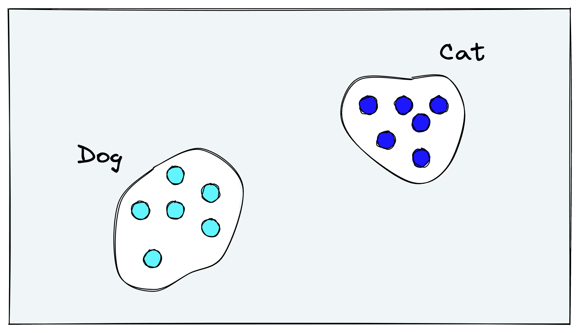
Retraining classification models is an option, but training requires significant time and capital investment for gathering a classification dataset and the act of model training itself.
Fortunately, OpenAI’s CLIP has proved itself as an incredibly flexible classification model that often requires zero retraining. In this chapter, we will explore zero-shot image classification using CLIP.
N-Shot Learning
Before diving into CLIP, let’s take a moment to understand what exactly “zero-shot” is and its significance in ML.
The concept derives from N-shot learning. Here we define N as the number of samples required to train a model to begin making predictions in a new domain or on a new task.
Many SotA models today are pretrained on vast amounts of data like ResNet or BERT. These pretrained models are then fine-tuned for a specific task and domain. For example, a ResNet model can be pretrained with ImageNet and then fine-tuned for clothing categorization.
Models like ResNet and BERT are called “many-shot” learners because we need many training samples to reach acceptable performance during that final fine-tuning step.
Many-shot learning is only possible when we have compute, time, and data to allow us to fine-tune our models. Ideally, we want to maximize model performance while minimizing N-shot requirements.
Zero-shot is the natural best-case scenario for a model as it means we require zero training samples before shifting it to a new domain or task.
CLIP may not be breaking SotA performance benchmarks on specific datasets. Still, it is proving to be a massive leap forward in zero-shot performance across various tasks in both image and text modalities.
The point of CLIP is not SotA performance. However, it’s worth noting that CLIP did beat the previous SotA results on the STL10 benchmark despite never being trained on that dataset.
The zero-shot adaptability of CLIP was found to work across many domains and different tasks. We will be talking about image classification in this article, but it can also be used in multi-modal search/recommendation, object detection, and likely many more as of yet unknown tasks.
How CLIP Makes Zero-Shot So Effective?
Contrastive Language-Image Pretraining (CLIP) is a primarily transformer-based model released by OpenAI in 2021 [1].
CLIP consists of two models, as discussed in more depth in the previous chapter. The version of CLIP we use here consists of a text transformer for encoding text embeddings and a vision transformer (ViT) for encoding image embeddings.
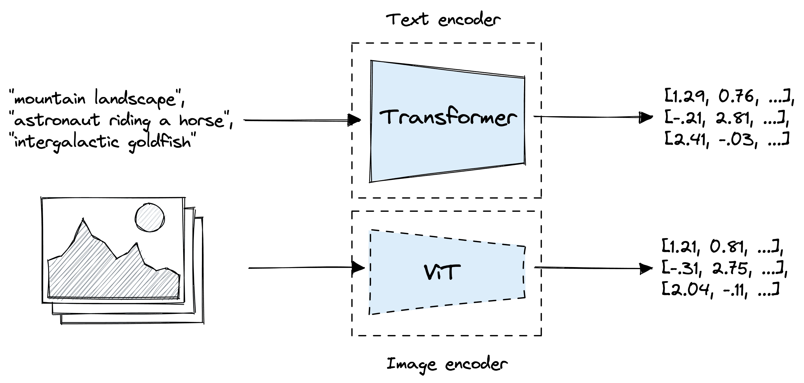
Both CLIP models are optimized during pretraining to align similar text and images in vector space. It does this by taking image-text pairs and pushing their output vectors nearer in vector space while separating the vectors of non-pairs.

It distinguishes itself from typical classification models for several reasons. First, OpenAI trained it on a huge dataset of 400M text-image pairs that were scraped from across the internet.
There are three primary benefits here:
- CLIP requires just image-text pairs rather than specific class labels thanks to the contrastive rather than classification focused training function. This type of data is abundant in today’s social-media-centric world.
- The large dataset size means CLIP can build a strong understanding of general textual concepts displayed within images.
- Text descriptors often describe various features of an image, not just one. Meaning a more holistic representation of images (and text) can be built.
These benefits of CLIP are the primary factors that have led to its outstanding zero-shot performance.
The authors of CLIP draw a great example of this by comparing a ResNet-101 model trained specifically on ImageNet to CLIP when both are applied to other datasets derived from ImageNet.
![ResNet-101 fine-tuned on ImageNet vs. zero-shot CLIP, source [1].](https://www.pinecone.io/_next/image/?url=https%3A%2F%2Fcdn.sanity.io%2Fimages%2Fvr8gru94%2Fproduction%2Fe58fd51aacd84d301d1cad0bb13dcd5296beb4df-2486x1398.png&w=3840&q=75)
ResNet-101 fine-tuned on ImageNet vs. zero-shot CLIP, source [1].
In this comparison, we can see that despite ResNet-101 training for ImageNet, its performance on similar datasets is much worse than CLIP on the same tasks. CLIP outperforms a SotA model trained for ImageNet on slightly modified ImageNet tasks.
When applying a ResNet model to other domains, a standard approach is to use a “linear probe”. That is where the ResNet learned features (from the last few layers) are fed into a linear classifier that is then fine-tuned for a specific dataset. We would regard this as few to many-shot learning.
In the CLIP paper, linear probe ResNet-50 was compared to zero-shot CLIP. In one scenario, zero-shot CLIP outperforms linear probing across many tasks.
![Zero-shot CLIP performance compared to ResNet with linear probe, source [1].](https://www.pinecone.io/_next/image/?url=https%3A%2F%2Fcdn.sanity.io%2Fimages%2Fvr8gru94%2Fproduction%2F86c758f560e227b83e43813377754a54265cdf49-521x554.png&w=1080&q=75)
Zero-shot CLIP performance compared to ResNet with linear probe, source [1].
Despite CLIP not being trained for these specific tasks, it outperforms a ResNet-50 with a linear probe. However, it’s worth noting that zero-shot did not outperform linear probing when given more training samples.
Zero-Shot Classification
How exactly does CLIP do zero-shot classification? We know that the image and text encoder creates a 512-dimensional image and text vector that map to the same vector space.
Considering this vector space alignment, what if we wrote the dataset classes as text sentences?
Given a task where we must identify whether a photo contains a car, bird, or cat: we could create and encode three text classes:
"a photo of a car" -> T_1 "a photo of a bird" -> T_2 "a photo of a cat" -> T_3
Each of these “classes” are output from the text encoder as vectors , , and respectively. Given an photo of a cat, we encode it with the ViT model to create vector . When we calculate the similarity of these vectors with cosine similarity, we expect to return the highest score.
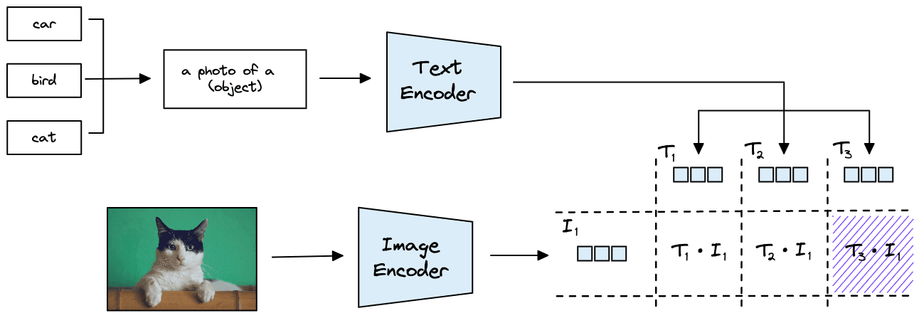
We reformat the one-word classes into sentences and encode them into label-based text vectors. When we encode and compare an image of a cat, we expect to share the highest similarity with *"a photo of a cat"*.
We format the one-word classes into sentences because we expect CLIP saw more sentence-like text during pretraining. For ImageNet it was reported that a 1.3 percentage point improvement in accuracy was achieved using the same prompt template of "a photo of a {label}" [1].
Prompt templates don’t always improve performance and they should be tested for each dataset. For the dataset we use below, we found it to reduce performance by 1.5 percentage points.
Python Implementation
Let’s move on to an applied example of CLIP for zero-shot classification. We will use the frgfm/imagenette dataset via Hugging Face Datasets.
In[2]:
# import the imagenette dataset
from datasets import load_dataset

imagenette = load_dataset(
    'frgfm/imagenette',
    '320px',
    split='validation',
    revision="4d512db"
)
# show dataset info
imagenette
Out[2]:
Dataset({
    features: ['image', 'label'],
    num_rows: 3925
})
In[3]:
# check labels in the dataset
set(imagenette['label'])
Out[3]:
{0, 1, 2, 3, 4, 5, 6, 7, 8, 9}The dataset contains 10 labels, all stored as integer values. To perform classification with CLIP we need the text content of these labels. Most Hugging Face datasets include the mapping to text labels inside the the dataset info:
In[4]:
# labels names
labels = imagenette.info.features['label'].names
labels
Out[4]:
['tench',
 'English springer',
 'cassette player',
 'chain saw',
 'church',
 'French horn',
 'garbage truck',
 'gas pump',
 'golf ball',
 'parachute']
In[5]:
# generate sentences
clip_labels = [f"a photo of a {label}" for label in labels]
clip_labels
Out[5]:
['a photo of a tench',
 'a photo of a English springer',
 'a photo of a cassette player',
 'a photo of a chain saw',
 'a photo of a church',
 'a photo of a French horn',
 'a photo of a garbage truck',
 'a photo of a gas pump',
 'a photo of a golf ball',
 'a photo of a parachute']
Before we can compare labels and photos, we need to initialize CLIP. We will use the CLIP implementation found via Hugging Face transformers.
In[6]:
# initialization
from transformers import CLIPProcessor, CLIPModel

model_id = "openai/clip-vit-base-patch32"

processor = CLIPProcessor.from_pretrained(model_id)
model = CLIPModel.from_pretrained(model_id)
In[7]:
import torch

# if you have CUDA set it to the active device like this
device = "cuda" if torch.cuda.is_available() else "cpu"
# move the model to the device
model.to(device)

device
Text transformers cannot read text directly. Instead, they need a set of integer values known as token IDs (or input_ids), where each unique integer represents a word or sub-word (known as a token).
We create these token IDs alongside another tensor called the attention mask (used by the transformer’s attention mechanism) using the processor we just initialized.
In[8]:
# create label tokens
label_tokens = processor(
    text=clip_labels,
    padding=True,
    images=None,
    return_tensors='pt'
).to(device)

label_tokens['input_ids'][0][:10]
Out[8]:
tensor([49406, 320, 1125, 539, 320, 1149, 634, 49407])Using these transformer-readable tensors, we create the label text embeddings like so:
In[9]:
# encode tokens to sentence embeddings
label_emb = model.get_text_features(**label_tokens)
# detach from pytorch gradient computation
label_emb = label_emb.detach().cpu().numpy()
label_emb.shape
In[10]:
label_emb.min(), label_emb.max()The vectors that CLIP outputs are not normalized, meaning dot product similarity will give inaccurate results unless the vectors are normalized beforehand. We do that like so:
In[11]:
import numpy as np

# normalization
label_emb = label_emb / np.linalg.norm(label_emb, axis=0)
label_emb.min(), label_emb.max()
(Alternatively, you can use cosine similarity)
All we have left is to work through the same process with the images from our dataset. We will test this with a single image first.
Out[12]:
<PIL.JpegImagePlugin.JpegImageFile image mode=RGB size=328x320 at 0x17F1B1A90>In[13]:
image = processor(
    text=None,
    images=imagenette[0]['image'],
    return_tensors='pt'
)['pixel_values'].to(device)
image.shape
Out[13]:
torch.Size([1, 3, 224, 224])After processing the image, we return a single (1) three-color channel (3) image width of 224 pixels and a height of 224 pixels. We must process incoming images to normalize and resize them to fit the input size requirements of the ViT model.
We can create the image embedding with:
In[14]:
img_emb = model.get_image_features(image)
img_emb.shape
In[15]:
img_emb = img_emb.detach().cpu().numpy()From here, all we need to do is calculate the dot product similarity between our image embedding and the ten label text embeddings. The highest score is our predicted class.
In[16]:
scores = np.dot(img_emb, label_emb.T)
scores.shape
In[17]:
# get index of highest score
pred = np.argmax(scores)
pred
In[18]:
# find text label with highest score
labels[pred]
Label 2, i.e., “cassette player” is our correctly predicted winner. We can repeat this logic over the entire frgfm/imagenette dataset to get the classification accuracy of CLIP.
In[19]:
from tqdm.auto import tqdm

preds = []
batch_size = 32

for i in tqdm(range(0, len(imagenette), batch_size)):
    i_end = min(i + batch_size, len(imagenette))
    images = processor(
        text=None,
        images=imagenette[i:i_end]['image'],
        return_tensors='pt'
    )['pixel_values'].to(device)
    img_emb = model.get_image_features(images)
    img_emb = img_emb.detach().cpu().numpy()
    scores = np.dot(img_emb, label_emb.T)
    preds.extend(np.argmax(scores, axis=1))
Out[19]:
0%| | 0/123 [00:00<?, ?it/s]In[20]:
true_preds = []
for i, label in enumerate(imagenette['label']):
    if label == preds[i]:
        true_preds.append(1)
    else:
        true_preds.append(0)

sum(true_preds) / len(true_preds)
That gives us an impressive zero-shot accuracy of 98.7%. CLIP proved to be able to accurately predict image classes with little more than some minor reformating of text labels to create sentences.
Zero-shot image classification with CLIP is a fascinating use case for high-performance image classification with minimal effort and zero fine-tuning required.
Before CLIP, this was not possible. Now that we have CLIP, it is almost too easy. The multi-modality and contrastive pretraining techniques have enabled a technological leap forward.
From multi-modal search, zero-shot image classification, and object detection to industry-changing tools like OpenAI’s Dall-E and Stable Diffusion, CLIP has opened the floodgates to many new use-cases that were previously blocked by insufficient data or compute.
Resources
[1] A. Radford, et. al., Learning Transferable Visual Models From Natural Language Supervision (2021)
Was this article helpful?