








Vector databases are emerging as a core part of the AI tech stack, serving knowledge to large language models (LLMs). A crucial part of vector databases is the ANN algorithms they use to index data, as they can affect query performance, including recall, latency, and the system's overall cost. This article will give an overview of the vector indexing landscape and analyses of a few popular algorithms.
Indexing structures, usually a collection of algorithms, consist of two components. The first is the algorithm for updating data: how inserts, deletes, and updates change the structure. The goal here is to put as little effort into creating a useful structure for searching as possible. The second is the algorithm for searching: search algorithms use the structure created during updates to find vectors relevant to the target query.
Algorithms don’t exist alone. We can only analyze their performance in the context of broader systems. An important framework for analyzing indexing algorithms is their interaction with storage media. Different algorithms work better or worse depending on the access characteristics of the media on which they are stored.
Storage media are generally viewed as having a hierarchy, where things high up in the hierarchy cost more but have higher performance, as shown in the diagram below. The three we will focus on are main memory, flash disk, and remote secondary storage (cloud object storage). At a high level, these have the following properties:
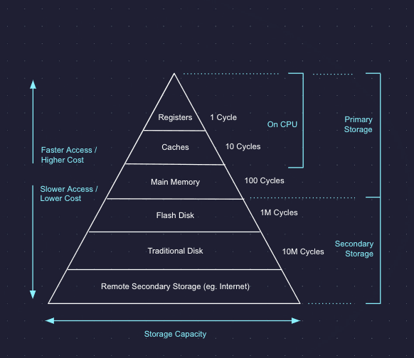
Storage media overview
With this in mind, let’s examine the main types of algorithms and how they utilize different storage media.
Based on how vectors are structured, vector indexing algorithms can be divided into three main categories:
We’ll skip hash-based indexing in this article because its performance on all aspects, including reads, writes, and storage, is currently worse than that of graph-based and spatial partitioning-based indexing. Almost no vector databases use hash-based indexing nowadays.
A spatial partitioning index organizes data into regions. Vectors are stored alongside other nearby vectors in the same region of space. Each partition is represented by a representative point, usually the centroid of the data points stored in the partition. Queries operate in two stages: first, they find the representative points closest to them. Then, they scan those partitions (see the example below, wherein a query at the red x).
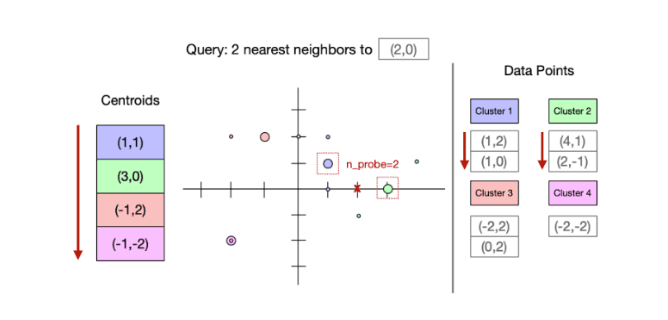
Spatial partitioning
Because points in a region are stored contiguously, partitioning indexes tend to make longer sequential reads than graph indexes. These types of indexes generally have a low storage footprint and are fast for writes. They work well with mediums that have higher bandwidth.
Spatial partitioning indexing has several benefits. First, they have very little space overhead. The structures they create for updating data and querying consist of representative points. There are far fewer centroids than actual vectors, reducing the space overhead.
Second, they can work well with object storage as they tend to make fewer, longer sequential reads than graph indexes.
However, they have lower query throughput than graph-based indexes in memory and on disk.
You can read this paper to learn more about spatial-partitioning indexing.
As their name suggests, graph-based indexes organize data as a graph. Reads start at an entry point and work by traversing the graph greedily by performing a best-first search. In particular, the algorithm keeps a priority queue of bounded size m, containing promising points whose neighbors haven’t been viewed yet. At each step, the algorithm takes the unexpanded point closest to the query and looks at its neighbors, adding any points closer than the current mth closest point onto the priority queue. The search stops when the queue contains only points whose neighbors have been expanded.
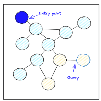
Graph-based indexing
Graph indexing algorithms have been shown empirically to have the best algorithmic complexity in terms of computation, in that they compute the distance to the fewest number of points to achieve a certain recall. As a result, they tend to be the fastest algorithms for in-memory vector search. Additionally, they can be engineered to work well on SSDs, so that they make only a small number of read requests. They are amongst the fastest algorithms for data that lie on SSDs.
One major difference is that the graph-based algorithm is sequential. It makes hops along the graph, and each hop is a small read. Thus, graphs do well with storage mediums that have low latency such as in-memory. They will not work in object storage as sequential reads of small items are too slow and object storage has high latency for read requests. Additionally, they have two other cons. First, each data point in a graph holds multiple edges, so they take more space to store than partitioning-based indexes. Second, inserts or deletes touch multiple nodes in the graph, and they tend to have higher costs for updates, especially for storage mediums with latency.
One complexity of discussing index types is that indexes can be a mix of types. The diagram below shows one of the most common mixed indexes.
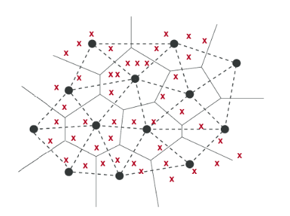
Mixed-index types
Here, the vectors (shown as red crosses) are organized into spatial partitions (shown by the solid black boundaries). The solid black points are the representative points of each partition. In step one of querying spatial partitioning-based indexes, we need to find the closest points amongst the representative points to decide which partitions to examine.
Since this is a nearest neighbor search itself, one can also index the representative points. And as there are fewer of these, it is easier to pay the price to store them in more expensive storage media like memory, and to store neighbors for each point. Thus a common technique is to index the representative points using a graph, taking advantage of the benefits of its higher read throughput, while leaving base data spatially partitioned and stored in contiguous arrays.
In general, we can categorize mixed indexing types by how their base points are stored. Base points are the vectors stored, as opposed to centroids, which are indexing structures. If every point is in the graph, it is graph-based indexing; if items are stored in files/arrays partitioned by space, it is spatial partitioning. Thus, we characterize indexes like SPANN, which has a graph on the centroids but uses spatial partitioning, as partitioning-based.
One of the most popular algorithms is Hierarchical Navigable Small Worlds (HNSW). It is the main indexing algorithm that most vector search solutions use.
We previously discussed that HNSW offers great recall at high throughput. Like many graph-based algorithms, HNSW is fast, getting its speed from its layered, hierarchical graph structure. Its nodes and edges connect semantically similar content, making it easy to find the most relevant vectors to a user’s query once within a target neighborhood, offering good recall.
However, HNSW can have high update costs and does not do well with production applications with dynamic data. Additionally, HNSW’s memory consumption grows quickly with data, which increases the cost of storing data in RAM and leads to higher query latencies, timeouts, and a higher bill.
Another popular index is the Inverted File Index (IVF). It’s easy to use, has high search quality, and has reasonable search speed.
It’s the most basic version of the spatial-partitioning index and inherits its advantages including little space overhead and the ability to work with object storage as well as disadvantages like lower query throughput compared to graph-based indexing in-memory and on-disk.
DiskANN is a graph-based index, that despite its name, can be designed for entirely in memory use cases or for data on SSD use cases. It is a leading graph algorithm and shares benefits and drawbacks that most graphs possess. In particular, across both data in memory and data on SSD use cases, it has high throughput. However, its high memory cost can make in RAM use cases expensive and on disk it can have high update overheads.
SPANN is a spatial partitioning based index meant for use with data on SSD. It puts a graph index over the set of representative points used for partitioning.
It’s good for disk-based nearest-neighbor searches, being faster than DiskANN at lower recalls (when both have the same recall) but slower at higher recalls. In general, it can be faster to update than DiskANN. However, updates can change the distribution of data, and more research is needed to see how robust it is in production for updates.
Vector indexing algorithms are complicated. We hope this article helps you understand the information needed when you’re learning and evaluating vector databases. In our upcoming content, we will share more about the Pinecone serverless algorithm. In the meantime, try Pinecone out for free.
此内容由惯性聚合(RSS阅读器)自动聚合整理,仅供阅读参考。 原文来自 — 版权归原作者所有。