







Have you ever wondered what happens under the hood when you train a neural network? You’ll run the gradient descent optimization algorithm to find the optimal parameters (weights and biases) of the network. In this process, there’s a loss function that tells the network how good or bad its current prediction is. The goal of optimization is to find those parameters that minimize the loss function: the lower the loss, the better the model.
In classification problems, the model predicts the class label of an input. In such problems, you need metrics beyond accuracy. While accuracy tells the model whether or not a particular prediction is correct, cross-entropy loss gives information on how correct a particular prediction is. When training a classifier neural network, minimizing the cross-entropy loss during training is equivalent to helping the model learn to predict the correct labels with higher confidence.
In this tutorial, we’ll go over binary and categorical cross-entropy losses, used for binary and multiclass classification, respectively. We’ll learn how to interpret cross-entropy loss and implement it in Python. As the loss function’s derivative drives the gradient descent algorithm, we’ll learn to compute the derivative of the cross-entropy loss function.
Let’s begin!
Before we proceed to learn about cross-entropy loss, it’d be helpful to review the definition of cross entropy. In the context of information theory, the cross entropy between two discrete probability distributions is related to KL divergence, a metric that captures how close the two distributions are.
Given a true distribution t and a predicted distribution p, the cross entropy between them is given by the following equation.
Here, both t and p are distributed on the same support S, but could take potentially different values. For a three-element support S, if t = [t1, t2, t3] and p = [p1, p2, p3], it’s not necessary that t_i = p_i for i in {1,2,3}.
Note: log(x) refers to log to the base e (or natural logarithm), also written as ln(x).
So how is cross entropy relevant in neural networks?
Recall that in binary classification, the sigmoid activation is used in the output layer, and the neural network outputs a probability score (p) between 0 and 1; the true label (t) being one of {0, 1}.
In case of multiclass classification, we use the softmax activation at the output layer to get a vector of predicted probabilities p. The true distribution t contains all of the probability mass (1) at the index of the correct class, and 0 everywhere else. For example, in a classification problem with N classes, the true distribution corresponding to class i is a vector that’s N classes long, with 1 at the index of the class label i and 0 at all other indices.
We’ll discuss this in greater detail in the coming sections.
Let’s start this section by reviewing the log function in the interval (0,1].
▶️ Run the following code snippet to plot the values of log(x) and -log(x) in the range 0 to 1. As log(0) is -∞, we add a small offset, and start with 0.001 as the smallest value in the interval.
import numpy as np
import seaborn as sns
from matplotlib import pyplot as plt
sns.set()
x_arr = np.linspace(0.001,1)
log_x = np.log(x_arr)
fig, axes = plt.subplots(1, 2,figsize=(8,4))
sns.lineplot(ax=axes[0],x=x_arr,y=log_x)
axes[0].set_title('Plot of log(x) in the interval (0,1]')
axes[0].set(xlabel='x', ylabel='log(x)')
sns.lineplot(ax=axes[1],x=x_arr,y=-log_x)
axes[1].set_title('Plot of -log(x) in the interval (0,1]')
axes[1].set(xlabel='x', ylabel='-log(x)')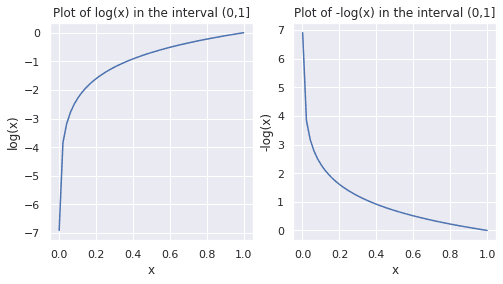
Plot of log x and -log x in the interval (0,1]
As seen in the plots above, in the interval (0,1], log(x) and -log(x) are negative and positive, respectively. Observe how -log(x) approaches 0 as x approaches 1. This observation will be helpful when we parse the expression for cross-entropy loss.
In binary classification, the raw output of the neural network is passed through the sigmoid function, which outputs a probability score p = σ(z), as shown below.
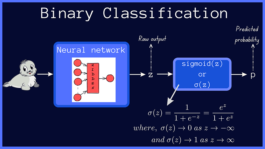
A Simple Binary Classification Model (Image by the author)
The true value, or the true label, is one of {0, 1} and we’ll call it t. The binary cross-entropy loss, also called the log loss, is given by:
As the true label is either 0 or 1, we can rewrite the above equation as two separate equations.
When t = 1, the second term in the above equation goes to zero, and the equation reduces to the following:
Therefore, when t =1, the binary cross-entropy loss is equal to the negative logarithm of the predicted probability p.
Similarly, when the true label t=0, the term t.log(p) vanishes, and the expression for binary cross-entropy loss reduces to:
Now, let’s plot the binary cross-entropy loss for different values of the predicted probability p.
bce_1 = -np.log(p)
bce_0 = -np.log(1-p)
plot1 = sns.lineplot(x=p,y=bce_1,label='True value:1').set(ylim=(0,4))
plot2 = sns.lineplot(x=p,y=bce_0,label='True value:0').set(ylim=(0,4))
plt.xlabel('p')
plt.ylabel('Binary Cross-Entropy Loss')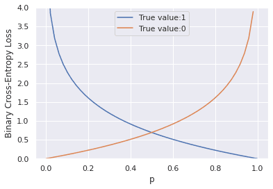
From the plots above, we can make the following observations:
t is 1, the cross-entropy loss approaches 0 as the predicted probability p approaches 1 andt is 0, the cross-entropy loss approaches 0 as the predicted probability p approaches 0.In essence, the cross-entropy loss attains its minimum when the predicted probability p is close to the true value and is substantially higher when the predicted probability is far away from the true label.
But which predictions does cross-entropy loss penalize the most?
Recall that log(0) → -∞; so -log(0) → ∞. As seen from the plots of the binary cross-entropy loss, this happens when the network outputs p=1 or a value close to 1 when the true class label is 0, and outputs p=0 or a value close to 0 when the true label is 1.
Putting it all together, cross-entropy loss increases drastically when the network makes incorrect predictions with high confidence.
If there are S samples in the dataset, then the total cross-entropy loss is the sum of the loss values over all the samples in the dataset.
Let’s define a Python function to compute the binary cross-entropy loss.
def binary_cross_entropy(t,p):
    t = np.float_(t)
    p = np.float_(p)
    # binary cross-entropy loss
    return -np.sum(t * np.log(p) + (1 - t) * np.log(1 - p))
Next, let’s call the function binary_cross_entropy with arrays of true and predicted values as the arguments.
t = [0,1,1,0,0,1,1]
p = [0.07,0.91,0.74,0.23,0.85,0.17,0.94]

binary_cross_entropy(t,p)
4.460303459760249
To get a better idea of how the loss varies with p, let’s modify the function definition to print out the values of the loss for each of the samples, as shown below.
def binary_cross_entropy(t,p):
    t = np.float_(t)
    p = np.float_(p)
    for tt, pp in zip(t,p):
      print(f'true_val = {tt}, predicted_val = {pp}, loss = {-(tt * np.log(pp) + (1 - tt) * np.log(1 - pp))}')
    return -np.sum(t * np.log(p) + (1 - t) * np.log(1 - p))
Now that we’ve modified the function, let’s call the function yet again to check the outputs.
binary_cross_entropy(t,p)

# Output
true_val = 0.0, predicted_val = 0.07, loss = 0.0725706928348355
true_val = 1.0, predicted_val = 0.91, loss = 0.09431067947124129
true_val = 1.0, predicted_val = 0.74, loss = 0.3011050927839216
true_val = 0.0, predicted_val = 0.23, loss = 0.2613647641344075
true_val = 0.0, predicted_val = 0.85, loss = 1.897119984885881
true_val = 1.0, predicted_val = 0.17, loss = 1.7719568419318752
true_val = 1.0, predicted_val = 0.94, loss = 0.06187540371808753
4.460303459760249
In the above output, when the true and predicted values are closer, the cross-entropy loss is lower; the loss increases when the true and predicted values are different.
The highest value of the loss, 1.897, occurs when the network predicts a probability score of 0.85 corresponding to a true value of 0. Suppose the problem is to classify whether the given image is that of a seal or not. The model, in this case, is 85% confident that the image is a seal when it actually isn’t.
Similarly, the second highest value of the binary cross-entropy loss, 1.771 occurs when the network predicts a score of 0.17, significantly lower than the true value of 1. In the image classification example, this means that the model is only about 17% confident of the input image being a seal, when it actually is a seal.
This validates our earlier observation that the loss is higher when the predictions are away from the true values.
In the next section, let’s explore an extension of cross-entropy loss to the multiclass classification case.
Let’s formalize the setting we’ll consider. In a multiclass classification problem over N classes, the class labels are 0, 1, 2 through N - 1. The labels are one-hot encoded with 1 at the index of the correct label, and 0 everywhere else.
For example, in an image classification problem where the input image is one of {panda, seal, duck}, the class labels and the corresponding one-hot vectors are shown below.
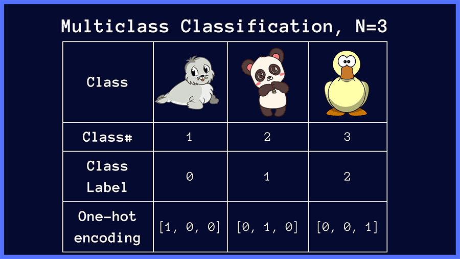
One-hot encoding of class labels in multiclass classification (Image by the author)
In multiclass classification, the raw outputs of the neural network are passed through the softmax activation, which then outputs a vector of predicted probabilities over the input classes.
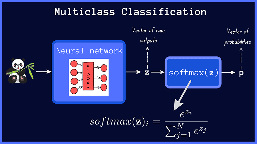
A Simple Multiclass Classification Model (Image by the author)
The categorical cross-entropy loss between the true distribution t and the predicted distribution p in a multiclass classification problem with N classes is given by:
This expression may seem daunting, but we’ll parse this and arrive at a much simpler expression.
Recall that the true distribution t is a one-hot vector that has 1 at one of the indices and zero everywhere else. If a given image belongs to the class k, in the true distribution vector, t_k = 1, and all other indices are zero.
Substituting as follows,
We see that N - 1 terms in the summation go to zero, and you’ll have the following simplified expression:
The loss, therefore, reduces to the negative logarithm of the predicted probability for the correct class. The loss approaches zero, as p_k → 1.
In the figure below, we present some examples of true and predicted distributions. In our image classification example, if the target class is seal, the categorical cross-entropy loss is minimized when the network predicts a probability score close to 1 for the correct class (seal). This works similarly for the other target classes, panda and duck.
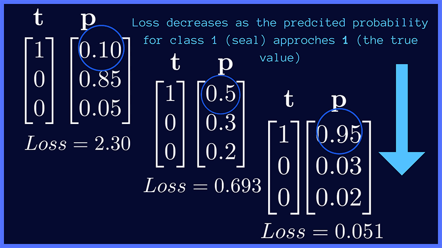
Cross-entropy loss decreases as the predicted probability for the target class approaches 1 (Image by the author)
For a dataset with S samples in all, the categorical cross-entropy loss is given by:
In practice, you could also use the average cross-entropy loss across all samples in the dataset. Next, let’s code the categorical cross-entropy loss in Python.
The code snippet below contains the definition of the function categorical_cross_entropy.The function accepts two lists as arguments: t_list and p_list containing lists of true and predicted distributions, respectively. It then computes the cross-entropy loss over each set of predicted and true values.
def categorical_cross_entropy(t_list,p_list):
    t_list = np.float_(t_list)
    p_list = np.float_(p_list)
    losses = []
    for t,p in zip(t_list,p_list):
      loss = -np.sum(t * np.log(p))
      losses.append(loss)
      print(f't:{t}, p:{p},loss:{loss}\n')
    return np.sum(losses)
Now, let’s make a call to the function with the lists of true and predicted distribution vectors as the arguments and check the outputs.
t_list = [[1,0,0],[0,1,0],[0,0,1],[1,0,0]]
p_list = [[0.91,0.04,0.05],[0.11,0.8,0.09],[0.3,0.1,0.6],[0.25,0.4,0.35]]
categorical_cross_entropy(t_list,p_list)

t:[1. 0. 0.], p:[0.91 0.04 0.05],loss:0.09431067947124129

t:[0. 1. 0.], p:[0.11 0.8  0.09],loss:0.2231435513142097

t:[0. 0. 1.], p:[0.3 0.1 0.6],loss:0.5108256237659907

t:[1. 0. 0.], p:[0.25 0.4  0.35],loss:1.3862943611198906

2.214574215671332
From the output above, we see that the loss is lower when the model predicts a higher probability corresponding to the correct class label.
One of the limitations of the argmax function as the output layer activation is that it doesn’t support the backpropagation of gradients through the layers of the neural network. However, when using the softmax function as the output layer activation, along with cross-entropy loss, you can compute gradients that facilitate backpropagation. The gradient evaluates to a simple expression, easy to interpret and intuitive.
If you’d like to know how softmax activation and cross-entropy loss yield a gradient that can be used in backpropagation, please read ahead. The preceding sections do not necessitate the use of the following section but this will provide interesting and potentially helpful insight.
The following subsections assume you have some familiarity with differential calculus. To follow along, you should be able to apply the chain rule for differentiation and compute partial derivatives.
Recall that if z is the output of the neural network, then softmax(z) outputs a vector p of probabilities. Let’s start with the expression for softmax activation.
Now, let’s compute the derivative of the softmax output p_i with respect to the raw output z_i of the neural network.
Here, the computation of derivatives can be handled under two different cases, as shown below.
Next, let’s compute the derivative of the cross-entropy loss function with respect to the output of the neural network. We’ll apply the chain rule and substitute the derivatives of the softmax activation function.
As seen above, the gradient works out to the difference between the predicted and true probability values.
In this tutorial, you’ve learned how binary and categorical cross-entropy losses work. They impose a penalty on predictions that are significantly different from the true value. You’ve learned to implement both the binary and categorical cross-entropy losses from scratch in Python. In addition, we covered how using the cross-entropy loss, in conjunction with the softmax activation, yields a simple gradient expression in backpropagation.
As a next step, you may try spinning up a simple image classification model using softmax activation and cross-entropy loss function. Until the next tutorial!
[1] Softmax Activation Function, pinecone.io
[2] Essence of Calculus, YouTube playlist by Grant Sanderson of 3Blue1Brown
[3] Gradient Descent Optimization, CS231n
[4] Backpropagation, CS231n
[5] Simple MNIST Convnet, keras.io
[6] Information Theory, Dive into Deep Learning
此内容由惯性聚合(RSS阅读器)自动聚合整理,仅供阅读参考。 原文来自 — 版权归原作者所有。