








When building language models, we can spend months optimizing training and model parameters, but it’s useless if we don’t have the correct data.
The success of our language models relies first and foremost on data. We covered a part way solution to this problem by applying the Augmented SBERT training strategy to in-domain problems. That is, given a small dataset, we can artificially enlarge it to enhance our training data and improve model performance.
In-domain assumes that our target use case aligns to that small initial dataset. But what if the only data we have does not align? Maybe we have Quora question duplicate pairs, but we want to identify similar questions on StackOverflow.
Given this scenario, we must transfer information from the out-of-domain (or source) dataset to our target domain. We will learn how to do this here. First, we will learn to assess which source datasets align best with our target domain quickly. Then we will explain and work through the AugSBERT domain-transfer training strategy [2].
Will it Work?
Before we even begin training our models, we can get a good approximation of whether the method will work with some simple n-gram matching statistics [1].
We count how many n-grams two different domains share. If our source domain shares minimal similarity to a target domain, as measured by n-gram matches, it is less likely to output good results.
This behavior is reasonably straightforward to understand; given our two source-target domains, overlapping n-grams indicate the linguistic and semantic gap (or overlap) between the two domains.
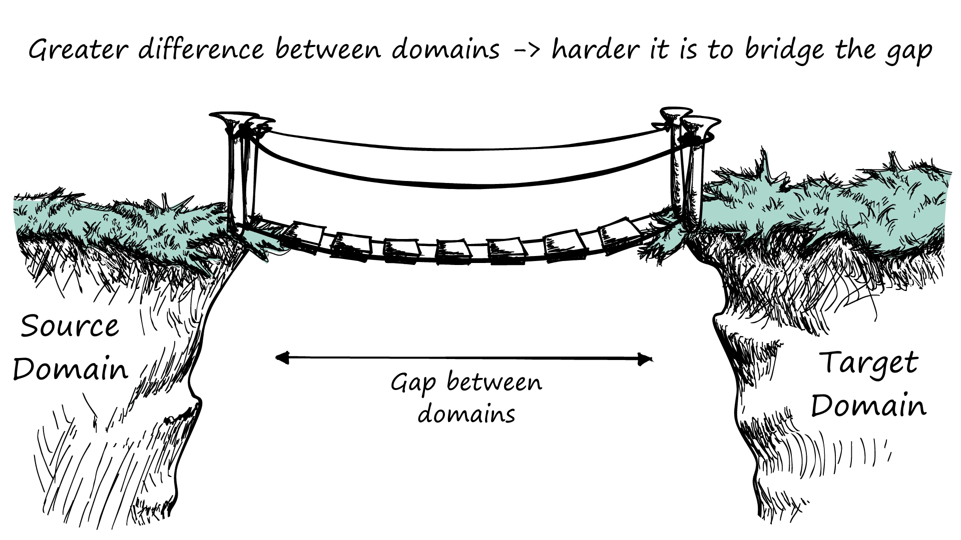
Small n-gram overlap indicates a more significant gap between domains. More significant gaps require larger bridges (better models). The closer the two domains, the easier it is to bridge the gap.
The greater the gap, the more difficult it is to bridge it using our training strategy. Although models are becoming better at generalization, they’re still brittle when compared to our human-level ability to adapt knowledge across domains.
The brittleness of language models means a small change can hamper performance. The more significant that change, the less likely our model will successfully translate its existing knowledge to the new domain.
We are similar. Although people are much more flexible and can apply pre-existing knowledge across domains incredibly well, we’re not perfect.
Given a book, we can tilt the pages at a slight five-degree angle, and most people will hardly notice the difference and continue reading. Turn the book upside-down, and many people will be unable to read. Others will begin to read slower. Our performance degrades with this small change.
If we are then given the same book in another language, most of us will have difficulty comprehending the book. It is still the same book, presented differently.
The knowledge transfer of models across different domains works in the same way: Greater change results in lower performance.
Calculating Domain Correlation
We will measure the n-gram overlap between five domains, primarily from Hugging Face Datasets.
| Dataset | Download Script |
|---|---|
| STSb | load_dataset('glue', 'stsb') |
| Quora Question Pairs (QQP) | load_dataset('glue', 'qqp') |
| Microsoft Research Paraphrase Corpus (MRPC) | load_dataset('glue', 'mrpc') |
| Recognizing Textual Entailment (RTE) | load_dataset('glue', 'rte') |
| Medical Question Pairs (Med-QP) | see below |
Link to Medical Question Pairs (Med-QP)
To calculate the similarity, we perform three operations:
- Tokenize datasets
In[1]:
from transformers import PreTrainedTokenizerFast

tokenizer = PreTrainedTokenizerFast.from_pretrained('bert-base-uncased')
In[2]:
text = "the quick brown fox jumped over the lazy dog"

tokens = tokenizer.tokenize(text)
tokens
Out[2]:
['the', 'quick', 'brown', 'fox', 'jumped', 'over', 'the', 'lazy', 'dog']- Merge tokens into bi-grams (two-token pairs)
In[3]:
ngrams = []
n = 2  # 2 for bigrams
for i in range(0, len(tokens), n):
    ngrams.append(' '.join(tokens[i:i+n]))
ngrams
Out[3]:
['the quick', 'brown fox', 'jumped over', 'the lazy', 'dog']- Calculate the Jaccard similarity between different n-grams.
In[4]:
# create new bigrams to compare against
ngrams_2 = ['the little', 'brown fox', 'is very',  'slow']
In[5]:
def jaccard (x: list, y: list):
    # convert lists to sets
    x = set(x)
    y = set(y)
    # calculate overlap
    shared = x.intersection(y)
    total = x.union(y)
    return len(shared) / len(total)
In[6]:
jaccard(ngrams, ngrams_2)After performing each of these steps and calculating the Jaccard similarity between each dataset, we should get a rough indication of how transferable models trained in one domain could be to another.
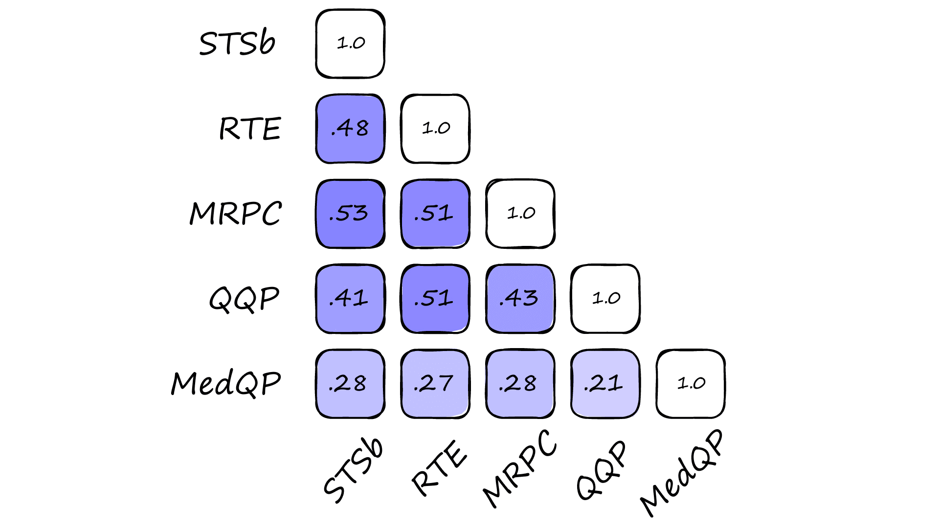
Jaccard similarity scores between each of the five datasets.
We can see that the MedQP dataset has the lowest similarity to other datasets. The remainder are all reasonably similar.
Other factors contribute to how well we can expect domain transfer to perform, such as the size of the source dataset and subsequent performance of the source cross encoder model within its own domain. We’ll take a look at these statistics soon.
Implementing Domain Transfer
The AugSBERT training strategy for domain transfer follows a similar pattern to that explained in our in-domain AugSBERT article. With the one exception that we train our cross-encoder in one domain and the bi-encoder (sentence transformer) in another.
At a high-level it looks like this:
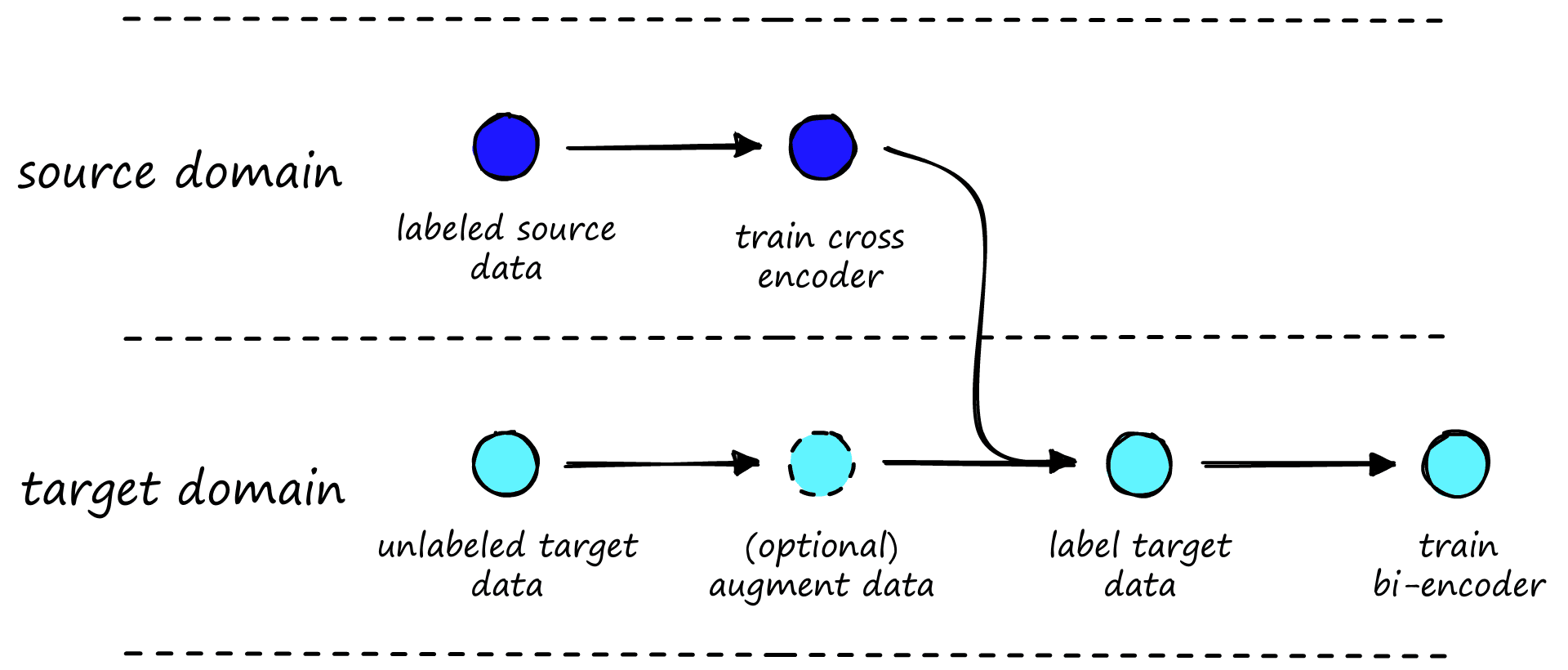
AugSBERT training strategy for cross-domain use.
We start with a labeled dataset from our source domain and an unlabeled dataset in our target domain. The source domain should be as similar as possible to our target domain.
The next step is to train the source domain cross-encoder. For this, we want to maximize cross encoder performance, as the bi-encoder will essentially learn to replicate the cross-encoder. Better cross-encoder performance translates to better bi-encoder performance.
If the target dataset is very small (1-3K pairs), we may need to augment the dataset. We do this because bi-encoder models require more data to be trained to the same level as a cross-encoder model. A good target dataset should contain 10K or more pairs, although this can vary by use case.
We label the previously unlabeled (and possibly augmented) target domain dataset with the trained cross-encoder.
The final step is to take the now labeled target domain data and use it to train the bi-encoder model.
That is all there is to it. We will add additional evaluation steps to confirm that the models are performing as expected, but otherwise, we’ll stick with the described process.
We already have our five datasets, and we will use each as both source and target data to see the difference in performance between domains.
When using a dataset for the target domain, we emulate a real-world use case (where we have no target data labels) by not including existing labels and instead relying solely on the cross-encoder-generated labels.
Cross Encoder Training
After downloading our labeled source data, we train the cross encoder. To do this, we need to format the source data into InputExample objects, then load them into a PyTorch DataLoader.
from sentence_transformers import InputExample
from torch.utils.data import DataLoader

data = []
# iterate through each row in dataset
for row in ds:
    # append InputExample object to the list
    data.append(InputExample(
        texts=[row['sentence1'], row['sentence2']],
        label=float(row['label'])
    ))

# initialize PyTorch DataLoader using data
source = DataLoader(
    data, shuffle=True, batch_size=16
)
It can be a good idea to take validation samples for either the source or target domains and create an evaluator that can be passed to the cross encoder training function. With this, the script will output Pearson and Spearman correlation scores that we can use to assess model performance.
from sentence_transformers.cross_encoder.evaluation import CECorrelationEvaluator

dev_data = []
# iterate through each row again (this time the validation split)
for row in dev:
    # build up using InputExample objects
    dev_data.append(InputExample(
        texts=[row['sentence1'], row['sentence2']],
        label=float(row['label'])
    ))

# the dev data goes into an evaluator
evaluator = CECorrelationEvaluator.from_input_examples(
    dev_data
)
To train the cross encoder model, we initialize a CrossEncoder and use the fit method. fit takes the source data dataloader, evaluator (optional), where we would like to save the trained model output_path, and a few training parameters.
# initialize the cross encoder
cross_encoder = CrossEncoder('bert-base-uncased', num_labels=1)

# setup the number of warmup steps, 0.2 == 20% warmup
num_epochs = 1
warmup = int(len(source) * num_epochs * 0.2)

cross_encoder.fit(
    train_dataloader=source,
    evaluator=evaluator,
    epochs=num_epochs,
    warmup_steps=warmup,
    optimizer_params={'lr': 5e-5},  # default 2e-5
    output_path=f'bert-{SOURCE}-cross-encoder'
)
For the training parameters, it is a good idea to test various learning rates and warm-up steps. A single epoch is usually enough to train the cross-encoder, and anything beyond this is likely to cause overfitting. Overfitting is bad when the target data is in-domain, and, when it is out-of-domain, it’s even worse.
For the five models being trained (plus one more trained on a restricted Quora-QP dataset containing 10K rather than 400K training pairs), the following learning rate and percentage of warm-up steps were used.
| Model | Learning Rate | Warmup | Evaluation (Spearman, Pearson) |
|---|---|---|---|
| bert-mrpc-cross-encoder | 5e-5 | 35% | (0.704, 0.661) |
| bert-stsb-cross-encoder | 2e-5 | 30% | (0.889, 0.887) |
| bert-rte-cross-encoder | 5e-5 | 30% | (0.383, 0.387) |
| bert-qqp10k-cross-encoder | 5e-5 | 20% | (0.688, 0.676) |
| bert-qqp-cross-encoder | 5e-5 | 20% | (0.823, 0.772) |
| bert-medqp-cross-encoder | 5e-5 | 40% | (0.737, 0.714) |
The Spearman and Pearson correlation values measure the correlation between the predicted and true labels for sentence pairs in the validation set. A value of 0.0 signifies no correlation, 0.5 is a moderate correlation, and 0.8+ represents strong correlation.
These results are fairly good, in particular the bert-stsb-cross-encoder and full bert-qqp-cross-encoder models return great performance. However, the RTE model bert-rte-cross-encoder performance is far from good.
The poor RTE performance is in part likely due to the small dataset size. However, as it is not significantly smaller than other datasets (Med-QP and MRPC in particular), we can assume the dataset is (1) not as clean or (2) that RTE is a more complex task.
| Dataset | Size |
|---|---|
| MRPC | 3,668 |
| STSb | 5,749 |
| RTE | 2,490 |
| Quora-QP | 363,846 |
| Med-QP | 2,753 |
We will find that this poor RTE performance doesn’t necessarily translate to poor performance in other domains. Indeed, very good performance in the source domain can actually hinder performance in the target domain because the model must be able to generalize well and not specialize too much in a particular domain.
We will later be taking a pretrained BERT model, which already has a certain degree of performance in the target domains. Overtraining in the source domain can pull the pretrained model alignment away from the target domain, hindering performance.
A better measure of potential performance is to evaluate against a small (or big if possible) validation set in the target domain.
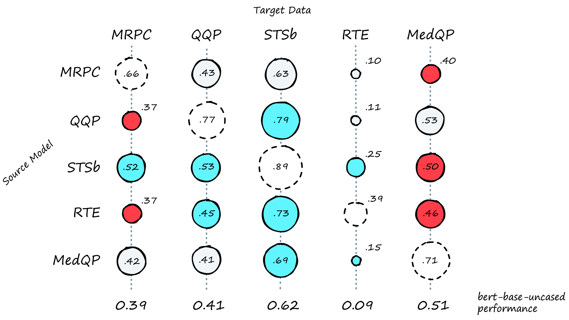
Correlation scores between source cross-encoder models (x-axis) and target domain dev sets (x-axis). The bottom row indicates baseline performance using a pretrained Bert-base-uncased model without fine-tuning. Lower scores are marked with red, above with cyan, and roughly equal with grey.
These correlation values are a good indication of the performance we can expect from our bi-encoder model. Immediately it is clear that the MedQP domain is not easily bridged as expected from the earlier n-gram analysis.
At this point, we can consider dropping the low performing source domains. Although we will keep them to see how these low cross-encoder scores translate to bi-encoder performance.
Labeling the Target Data
The next step is to create our labeled target dataset. We use the cross-encoder trained in the source domain to label the unlabeled target data.
This is relatively straightforward. We take the unlabeled sentence pairs, transform them into a list of sentence pairs, and feed them into the cross_encoder.predict method.
# target data is from the training sets from prev snippets
# (but we ignore the label feature, otherwise there is nothing to predict)
pairs = list(zip(target['sentence1'], target['sentence2']))

scores = cross_encoder.predict(pairs)
We return a set of similarity scores, which we can append to the target data and use it to train our bi-encoder.
import pandas as pd

# store everything in a pandas DataFrame
target = pd.DataFrame({
    'sentence1': target['sentence1'],
    'sentence2': target['sentence2'],
    'label': scores.tolist()  # cross encoder predicted labels
})
# and save to file
target.to_csv('target_data.tsv', sep='\t', index=False)
Training the Bi-Encoder
The final step in the training process is training the bi-encoder/sentence transformer itself. Everything we’ve done so far has been to label the target dataset.
Now that we have the dataset, we first need to reformat it using InputExample objects and a DataLoader as before.
from torch.utils.data import DataLoader
from sentence_transformers import InputExample

# create list of InputExamples
train = []
for i, row in target.iterrows():
  	train.append(InputExample(
      	texts=[row['sentence1'], row['sentence2']],
      	label=float(row['label'])
    ))
# and place in PyTorch DataLoader
loader = DataLoader(
  	train, shuffle=True, batch_size=BATCH_SIZE
)
Then we initialize the bi-encoder. We will be using a pretrained bert-base-uncased model from Hugging Face Transformers followed by a mean pooling layer to transform word-level embeddings to sentence embeddings.
In[7]:
from sentence_transformers import models, SentenceTransformer

# initialize model
bert = models.Transformer('bert-base-uncased')
# and mean pooling layer
pooler = models.Pooling(
    bert.get_word_embedding_dimension(),
    pooling_mode_mean_tokens=True
)
# then place them together
model = SentenceTransformer(modules=[bert, pooler])
model
Out[7]:
SentenceTransformer(
  (0): Transformer({'max_seq_length': 512, 'do_lower_case': False}) with Transformer model: BertModel
  (1): Pooling({'word_embedding_dimension': 768, 'pooling_mode_cls_token': False, 'pooling_mode_mean_tokens': True, 'pooling_mode_max_tokens': False, 'pooling_mode_mean_sqrt_len_tokens': False})
)
The labels output by our cross encoder are continuous values in the range 0.0 -> 1.0, which means we can use a loss function like CosineSimilarityLoss. Then we’re ready to train our model as we have done before.
# setup loss function
loss = losses.CosineSimilarityLoss(model=model)

# and training
epochs = 1
# warmup for first 30% of training steps (test diff values here)
warmup_steps = int(len(loader) * epochs * 0.3)

model.fit(
  train_objectives=[(loader, loss)],
  epochs=epochs,
  warmup_steps=warmup_steps,
  output_path=f'bert-target'
)
Evaluation and Augmentation
At this point, we can evaluate the bi-encoder model performance on a validation set of the target data. We use the EmbeddingSimilarityEvaluator to measure how closely the predicted, and true labels correlate (script here).
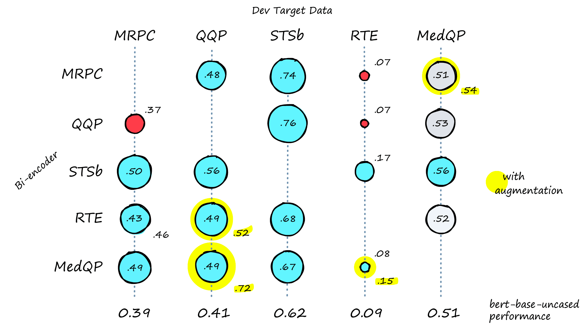
Bi-encoder correlation scores. Many reach very close to the equivalent cross-encoder performance (and some even exceed it). Yellow highlights indicate an improved performance after augmentation via random sampling.
The first bi-encoder results are reasonable, with most scoring higher than the Bert benchmark. Highlighted results indicate the original score (in the center) followed by scores after augmenting target datasets with random sampling. Where data augmentation showed little-to-no improvement, scores were excluded.
One reason we might see improvement is quite simple. Bi-encoders require relatively large training sets. Our datasets are all tiny, except for QQP (which does produce a 72% correlation score in bert-Smedqp-Tqqp). Augmented datasets help us satisfy the data-hungry nature of bi-encoder training.
Fortunately, we already set up most of what we needed to augment our target datasets. We have the cross-encoders for labeling, and all that is left is to generate new pairs.
As covered in our in-domain AugSBERT article, we can generate new pairs with random sampling. All this means is that we create new sentence pairs by mixing-and-matching sentences from features A and B.
After generating these new pairs, we score them using the relevant cross-encoder. And like magic, we have thousands of new samples to train our bi-encoders with.
With or without random sampling, we can see results that align with the performance of our cross-encoder models, which is precisely what we would expect. This similarity in results means that the knowledge from our cross-encoders is being distilled successfully into our faster bi-encoder models.
That is it for the Augmented SBERT training strategy and its application to domain transfer. Effective domain transfer allows us to broaden the horizon of sentence transformer use across many more domains.
The most common blocker for new language tools that rely on BERT or other transformer models is a lack of data. We do not eliminate the problem entirely using this technique, but we can reduce it.
Given a new domain that is not too far from the domain of existing datasets, we can now build better-performing sentence transformers. Sometimes in the range of just a few percentage point improvements, and at other times, we see much more significant gains.
Thanks to AugSBERT, we can now tackle a few of those previously inaccessible domains.
References
[1] D. Shah, et al., Adversarial Domain Adaption for Duplicate Question Detection (2018), EMNLP Proc.
[2] N. Thakur, et al., Augmented SBERT: Data Augmentation Method for Improving Bi-Encoders for Pairwise Sentence Scoring Tasks (2021), NAACL
Was this article helpful?