在数字信号处理和电子测量中，示波器是一种不可或缺的工具，用于观察和分析各种信号。然而，在实际应用中，为了准确地重建波形，我们需要理解并应用奈奎斯特定理以及适当的插值方法。本文将详细介绍奈奎斯特定理在示波器波形重建中的应用，并探讨正弦内插（Sine Interpolation）的具体实现。

奈奎斯特定理

奈奎斯特定理是数字信号处理中的一个基本原理，它指出：只要采样频率 \( f_s \) 大于或等于信号最高频率 \( f_m \) 的两倍，即 \( f_s \geq 2f_m \)，那么通过理想采样信号就可以不失真地恢复连续时间信号。如果信号的最高频率超过了 \( f_s / 2 \)，就会发生频谱混叠现象，使得用基带滤波器无法不失真地恢复信号。

数学上，奈奎斯特定理可以表示为：

\[ f_s \geq 2f_m \]

频谱混叠现象

当采样频率不满足奈奎斯特条件时，信号的高频成分会折叠到低频区域，导致频谱混叠。这种混叠使得信号的恢复变得困难，甚至不可能准确还原原始信号。

正弦内插在波形重建中的应用

在示波器的波形重建过程中，正弦内插是一种常用的技术，用于在实际采样点之间插入新的数据点，从而提高波形的平滑度和准确性。正弦内插的基本思想是利用正弦函数的平滑特性来生成中间的数据点。

正弦内插公式

假设我们有两个已知的数据点 \( (x_0, y_0) \) 和 \( (x_1, y_1) \)，我们希望在这两个点之间生成一系列新的数据点 \( (x_i, y_i) \)。正弦内插可以通过以下公式实现：

\[ y(t) = y_0 + (y_1 - y_0) \cdot \left( \frac{1 - \cos(\pi t)}{2} \right) \]

其中，\( t \) 是从0到1的线性参数。

信号通过理想低通滤波器的响应过程

理想低通滤波器的冲激响应 \( g(t) \) 可以表示为：

\[ g(t) = \frac{\sin(\pi t / T)}{\pi t / T} \]

根据卷积公式，通过低通滤波器的信号输出为：

\[ y(t) = \sum_{n=-\infty}^{\infty} x(nT) g(t - nT) \]

其中，\( g(t - nT) \) 称为内插函数。

采样内插公式

采样内插公式表明了连续时间信号 \( z(t) \) 如何由它的采样序列 \( x(nT) \) 来恢复：

\[ z(t) = \sum_{n=-\infty}^{\infty} x(nT) \frac{\sin(\pi (t - nT) / T)}{\pi (t - nT) / T} \]

这个公式的意义在于：只要满足了采样频率大于信号最高频率两倍的条件，整个连续时间信号 \( z(t) \) 可以由它的采样序列 \( x(nT) \) 恢复，而不丢失任何信息。

对于数字示波器来说，被测数字信号的频谱分量实际上是无穷的。为了确保一定的准确度，示波器或放大器的带宽应该是被测信号带宽的2倍（高斯频响示波器）或1.4倍（Flat频响示波器）。这样可以保证足够的频谱分量通过放大器。

• 高斯频响示波器：采样率应该是示波器带宽的4倍。
• Flat频响示波器：采样率应该是示波器带宽的2.5倍。

这些要求的原因是被测数字信号的频谱分量实际上是无穷的，放大器的滤波作用并非把-3dB带宽的带外信号全部滤掉，而是频响曲线上会拖个尾巴。因此，采样率应该包括尾巴部分的2倍以上，而非仅仅是一-3dB带宽的2倍以上。

频谱混叠的影响

如果采样率不能满足上述要求，就会发生频谱混叠，从而引起插值的错误，导致波形的失真。因此，选择合适的采样率和插值方法对于准确重建波形至关重要。

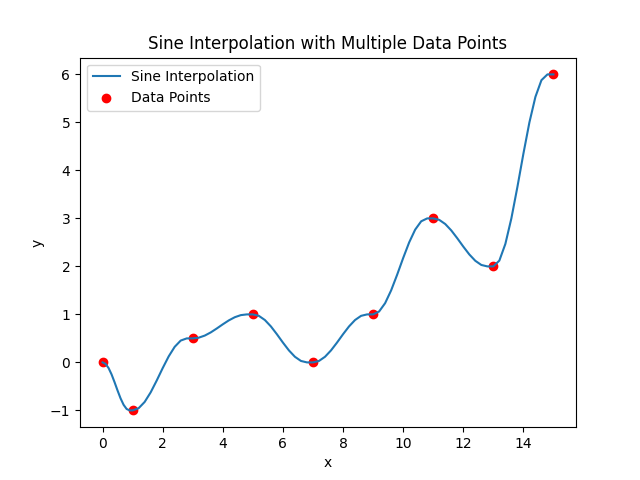
使用正弦内插法对采样点进行插值如下所示，可以观察到各个采样点中插值过渡平衡

# 正弦内插法示例代码
import numpy as np
import matplotlib.pyplot as plt


def sine_interpolation(y0, y1, num_points):
    t = np.linspace(0, 1, num_points)
    y = y0 + (y1 - y0) * (1 - np.cos(np.pi * t)) / 2
    return y

def interpolate_sequence(x, y, num_points_per_segment):
    interpolated_x = []
    interpolated_y = []

    for i in range(len(x) - 1):
        x0, x1 = x[i], x[i + 1]
        y0, y1 = y[i], y[i + 1]

        # 生成中间 x 值
        segment_x = np.linspace(x0, x1, num_points_per_segment, endpoint=False)
        interpolated_x.extend(segment_x)

        # 进行正弦内插
        segment_y = sine_interpolation(y0, y1, num_points_per_segment)
        interpolated_y.extend(segment_y)

    # 添加最后点
    interpolated_x.append(x[-1])
    interpolated_y.append(y[-1])

    return np.array(interpolated_x), np.array(interpolated_y)

# 示例数据点
x = np.array([0, 1, 3, 5, 7, 9])
y = np.array([0, -1, 0.5, 1, 0, 1])

# 每个段之间的内插点数
num_points_per_segment = 10

# 进行正弦内插
interpolated_x, interpolated_y = interpolate_sequence(x, y, num_points_per_segment)

# 绘制结果
plt.plot(interpolated_x, interpolated_y, label='Sine Interpolation')
plt.scatter(x, y, color='red', label='Data Points')
plt.xlabel('x')
plt.ylabel('y')
plt.title('Sine Interpolation with Multiple Data Points')
plt.legend()
plt.show()