





With the disadvantages of the KNN algorithm, we need to come up with a more powerful approach. The new approach will have two major components: a score function that maps the raw data to class scores, and a loss function that quantifies the agreement between the predicted scores and the ground truth labels.
The score function maps the pixel values of an image to confidence scores for each class.
As before, let’s assume a training dataset of images xi∈RD\mathbf{x}_i \in \mathbf{R}^D, each associated with a label yiy_i. Here i=1…Ni = 1 \dots N and yi∈1…Ky_i \in 1 \dots K.
That is, we have N\mathbf{N} examples (each with a dimensionality D\mathbf{D}) and K\mathbf{K} distinct categories.
We will define the score function f:RD↦RKf : \mathbf{R}^D \mapsto \mathbf{R}^K that maps the raw image pixels to class scores.
We will start out with arguably the simplest possible function, a linear mapping.
f(xi,W,b)=Wxi+bf(\mathbf{x}_i, \mathbf{W}, \mathbf{b}) = \mathbf{W}\mathbf{x}_i + \mathbf{b}
In the above equation, we are assuming that the image xi\mathbf{x}_i has all of its pixels flattened out to a single column vector of shape [D x 1]. The matrix W\mathbf{W} (of size [K x D]), and the vector b\mathbf{b} (of size [K x 1]) are the parameters of the function.
The parameters in W\mathbf{W} are often called the weights, and b\mathbf{b} is called the bias vector because it influences the output scores, but without interacting with the actual data xi\mathbf{x}_i.
The input data are given and fixed. The goal is to set W,b\mathbf{W,b} in such way that the computed scores match the ground truth labels across the whole training set.
We can combine the two sets of parameters into a single matrix that holds both of them by extending the vector xi\mathbf{x}_i with one additional dimension that always holds the constant 1\mathbf{1} - a default bias dimension.
f(xi,W)=Wxif(\mathbf{x}_i, \mathbf{W}) = \mathbf{W}\mathbf{x}_i
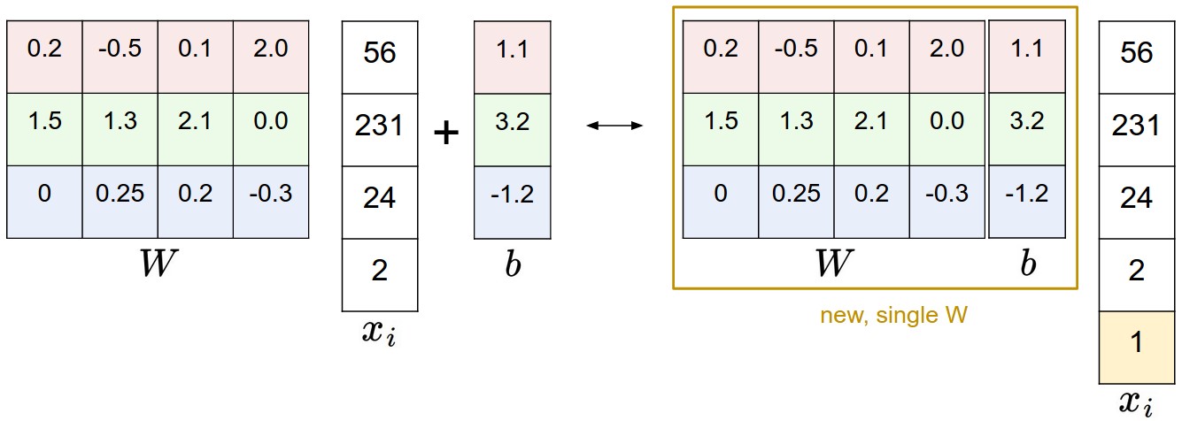
In Machine Learning, it is a very common practice to always perform normalization of input features. In particular, it is important to center your data by subtracting the mean from every feature.
We will develop Multiclass Support Vector Machine (SVM) loss.
The score function takes the pixels and computes the vector f(xi,W)f(\mathbf{x}_i, \mathbf{W}) of class scores, which we will abbreviate to s\mathbf{s} (short for scores).
The Multiclass SVM loss for the i-th example is then formalized as follows:
Li=∑j≠yimax(0,sj−syi+Δ)L_i = \sum_{j \neq y_i} \max(0, s_j - s_{y_i} + \Delta)
The function accumulates the error of incorrect classes within Delta.
In summary, the SVM loss function wants the score of the correct class yiy_i to be larger than the incorrect class scores by at least by Δ\Delta (delta).
The threshold at zero max(0, -) function is often called the hinge loss. We also have squared hinge loss SVM (or L2-SVM), which uses the form max(0, -)² that penalizes violated margins more strongly.

We wish to encode some preference for a certain set of weights W over others to remove this ambiguity. We can do so by extending the loss function with a regularization penalty R(W)R(\mathbf{W}). The most common regularization penalty is the squared L2 norm that discourages large weights through an elementwise quadratic penalty over all parameters:
R(W)=∑k∑lWk,l2R(\mathbf{W}) = \sum_k \sum_l W_{k,l}^2
Including the regularization penalty completes the full Multiclass Support Vector Machine loss, which is made up of two components: the data loss (which is the average loss LiL_i over all examples) and the regularization loss.
L=1N∑iLi⏟data loss+λR(W)⏟regularization lossL = \underbrace{\frac{1}{N} \sum_i L_i}_{\text{data loss}} + \underbrace{\lambda R(\mathbf{W})}_{\text{regularization loss}}
Or in full form:
L=1N∑i∑j≠yi[max(0,f(xi;W)j−f(xi;W)yi+Δ)]+λ∑k∑lWk,l2L = \frac{1}{N} \sum_i \sum_{j \neq y_i} \left[ \max(0, f(\mathbf{x}_i; \mathbf{W})_j - f(\mathbf{x}_i; \mathbf{W})_{y_i} + \Delta) \right] + \lambda \sum_k \sum_l W_{k,l}^2
Penalizing large weights tends to improve generalization, because it means that no input dimension can have a very large influence on the scores all by itself. It keeps the weights small and simple. This can improve the generalization performance of the classifiers on test images and lead to less overfitting.
It prevents the model from doing too well on the training data.
Note that due to the regularization penalty we can never achieve loss of exactly 0.0 on all examples.
Setting Delta: It turns out that this hyperparameter can safely be set to Δ=1.0\Delta = 1.0 in all cases. (The exact value of the margin between the scores is in some sense meaningless because the weights can shrink or stretch the differences arbitrarily.)
Binary Support Vector Machine: The loss for the i-th example can be written as
Li=Cmax(0,1−yiwTxi)+R(W)L_i = C \max(0, 1 - y_i \mathbf{w}^T \mathbf{x}_i) + R(\mathbf{W})
C\mathbf{C} in this formulation and λ\lambda in our formulation control the same tradeoff and are related through reciprocal relation C∝1λC \propto \frac{1}{\lambda}.
Other Multiclass SVM formulations: Multiclass SVM presented in this section is one of few ways of formulating the SVM over multiple classes.
Another commonly used form is the One-Vs-All (OVA) SVM which trains an independent binary SVM for each class vs. all other classes. Related, but less common to see in practice is also the All-vs-All (AVA) strategy.
The last formulation you may see is a Structured SVM, which maximizes the margin between the score of the correct class and the score of the highest-scoring incorrect runner-up class.
In the Softmax Classifier, we now interpret these scores as the unnormalized log probabilities for each class and replace the hinge loss with a cross-entropy loss that has the form:
Li=−log(efyi∑jefj)or equivalentlyLi=−fyi+log∑jefjL_i = -\log\left(\frac{e^{f_{y_i}}}{\sum_j e^{f_j}}\right) \hspace{1cm} \text{or equivalently} \hspace{1cm} L_i = -f_{y_i} + \log\sum_j e^{f_j}
where we are using the notation fjf_j to mean the j-th element of the vector of class scores f\mathbf{f}.
The function fj(z)=ezj∑kezkf_j(\mathbf{z}) = \frac{e^{z_j}}{\sum_k e^{z_k}} is called the softmax function: It takes a vector of arbitrary real-valued scores (in z\mathbf{z}) and squashes it to a vector of values between zero and one that sum to one.
The cross-entropy between a “true” distribution p\mathbf{p} and an estimated distribution q\mathbf{q} is defined as:
H(p,q)=−∑xp(x)logq(x)H(\mathbf{p}, \mathbf{q}) = -\sum_x p(x) \log q(x)
Minimizing Cross-Entropy is equivalent to minimizing the KL Divergence.
H(p,q)=H(p)+DKL(p∣∣q)H(p, q) = H(p) + D_{KL}(p||q)
Because the true distribution pp is fixed (its entropy H(p)H(p) is zero in this scenario), minimizing cross-entropy is the same as forcing the predicted distribution qq to look exactly like the true distribution pp.
The Softmax Loss objective is to force the neural network to output a probability distribution where the correct class has a probability very close to 1.0, and all other classes are close to 0.0.
Information Entropy measures the uncertainty or unpredictability of a random variable.
The more unpredictable an event is (lower probability), the more information is gained when it occurs, and the higher the entropy. Conversely, if an event has a probability of 1 (certainty), its entropy is 0.
For a discrete random variable XX with possible outcomes {x1,...,xn}\{x_1, ..., x_n\} and probabilities P(xi)P(x_i), the entropy H(X)H(X) is defined as:
H(X)=−∑i=1nP(xi)logP(xi)H(X) = -\sum_{i=1}^{n} P(x_i) \log P(x_i)
Cross Entropy measures the total cost of using distribution qq to represent distribution pp.
Minimizing the cross-entropy H(p,q)H(p, q) is mathematically equivalent to minimizing the KL Divergence. It forces the predicted distribution qq to become as close as possible to the true distribution pp.
P(yi∣xi;W)=efyi∑jefjP(y_i \mid x_i; W) = \frac{e^{f_{y_i}}}{\sum_j e^{f_j}}
The formula maps raw scores to a range of (0,1)(0, 1) such that the sum of all class probabilities equals 1.
Using the Cross-Entropy loss function during training is equivalent to maximizing the likelihood of the correct class.
Dividing large numbers can be numerically unstable, so it is important to use a normalization trick.
efyi∑jefj=CefyiC∑jefj=efyi+logC∑jefj+logC\frac{e^{f_{y_i}}}{\sum_j e^{f_j}} = \frac{Ce^{f_{y_i}}}{C\sum_j e^{f_j}} = \frac{e^{f_{y_i} + \log C}}{\sum_j e^{f_j + \log C}}
A common choice for CC is to set logC=−maxjfj\log C = -\max_j f_j. This simply states that we should shift the values inside the vector ff so that the highest value is zero. In code:
1 | f = np.array([123, 456, 789]) |
To be precise, the SVM classifier uses the hinge loss, or also sometimes called the max-margin loss.
The Softmax classifier uses the cross-entropy loss.
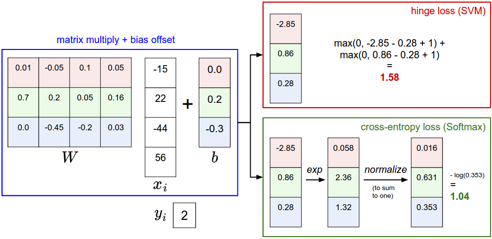
The SVM interprets these as class scores and its loss function encourages the correct class to have a score higher by a margin than the other class scores.
The Softmax classifier instead interprets the scores as (unnormalized) log probabilities for each class and then encourages the (normalized) log probability of the correct class to be high (equivalently the negative of it to be low).
Softmax classifier provides “probabilities” for each class.
The “probabilities” are dependent on the regularization strength. They are better thought of as confidences where the ordering of the scores is interpretable.
In practice, SVM and Softmax are usually comparable. Compared to the Softmax classifier, the SVM is a more local objective.
The Softmax classifier is never fully happy with the scores it produces: the correct class could always have a higher probability and the incorrect classes always a lower probability and the loss would always get better.
However, the SVM is happy once the margins are satisfied and it does not micromanage the exact scores beyond this constraint.
此内容由惯性聚合(RSS阅读器)自动聚合整理,仅供阅读参考。 原文来自 — 版权归原作者所有。