Batch normalization and layer normalization improve training stability and reduce sensitivity to initialization by normalizing intermediate activations.

When training a deep neural network, the distribution of inputs to each layer can change as the network’s weights are updated. If the weights become too large, the inputs to subsequent layers may grow excessively; if the weights shrink toward zero, the inputs may diminish accordingly. These shifts in input distributions make training more difficult, as each layer must continuously adapt to changing conditions. This phenomenon is known as internal covariate shift.

Normalization allows us to use much higher learning rates and be less careful about initialization.

Plain Normalization

If normalization (e.g., centering the activations to zero mean) is performed outside of the gradient descent step, the optimizer will remain “blind” to the normalization’s effects.

In formal terms, if the optimizer treats the mean-subtraction operation as a fixed constant, the gradient updates will fail to reflect the true dynamics of the network.

Consider a layer that computes x=u+bx = u + b and subsequently normalizes it: x^=x−E[x]\hat{x} = x - E[x].

If the gradient ∂ℓ∂b\frac{\partial \ell}{\partial b} is computed without considering how E[x]E[x] depends on bb, the optimizer will attempt to adjust bb to minimize the loss.

Because the normalization step subsequently subtracts the updated mean, the update Δb\Delta b is effectively cancelled. The output x^\hat{x} remains numerically identical to its state prior to the update:

(u+b+Δb)−E[u+b+Δb]=u+b−E[u+b](u + b + \Delta b) - E[u + b + \Delta b] = u + b - E[u + b]

Since the output—and consequently the loss—remains invariant despite the update, the optimizer will continue to increase bb in a futile attempt to reach a lower loss. This results in unbounded parameter growth while the network’s predictive performance stagnates.

To maintain training stability, normalization must be included within the computational graph so that gradients correctly capture its dependence on the parameters.

However, performing full whitening across all examples can be computationally expensive. This is why techniques like Batch Normalization and Layer Normalization are used instead.

Batch Normalization

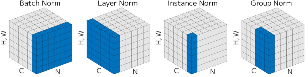
Batch Normalization performs normalization for each training mini-batch.

In Batch Normalization, we normalize each scalar feature independently, by making it have the mean of zero and the variance of 1.

x^(k)=x(k)−E[x(k)]Var[x(k)]+ϵ\hat{x}^{(k)} = \frac{x^{(k)} - \mathbb{E}[x^{(k)}]}{\sqrt{\mathrm{Var}[x^{(k)}] + \epsilon}}

But simply normalizing each input of a layer may change what the layer can represent. The authors make sure that the transformation inserted in the network can represent the identity transform. Thus introducing:

y(k)=γ(k)x^(k)+β(k)y^{(k)} = \gamma^{(k)} \hat{x}^{(k)} + \beta^{(k)}

The parameters here are learnable along with the original model parameters, and restore the representation power of the network.

By setting γ(k)=Var[x(k)]\gamma^{(k)} = \sqrt{\mathrm{Var}[x^{(k)}]} and β(k)=E[x(k)]\beta^{(k)} = \mathbb{E}[x^{(k)}], we could recover the original activations, if that were the optimal thing to do.

Algorithm 1: Batch Normalization Forward Pass

The forward pass of the Batch Normalization layer transforms a mini-batch of activations B={x1…m}\mathcal{B} = \{x_{1 \dots m}\} into a normalized and linearly scaled output {yi}\{y_i\}. This process ensures that the input to subsequent layers maintains a stable distribution throughout training.

Input: Values of xx over a mini-batch: B={x1…m}\mathcal{B} = \{x_{1 \dots m}\}; Parameters to be learned: γ,β\gamma, \beta.
Output: {yi=BNγ,β(xi)}\{y_i = \text{BN}_{\gamma, \beta}(x_i)\}.

1. Mini-batch Mean:

μB←1m∑i=1mxi\mu_{\mathcal{B}} \leftarrow \frac{1}{m} \sum_{i=1}^m x_i

2. Mini-batch Variance:

σB2←1m∑i=1m(xi−μB)2\sigma_{\mathcal{B}}^2 \leftarrow \frac{1}{m} \sum_{i=1}^m (x_i - \mu_{\mathcal{B}})^2

3. Normalize:

x^i←xi−μBσB2+ϵ\hat{x}_i \leftarrow \frac{x_i - \mu_{\mathcal{B}}}{\sqrt{\sigma_{\mathcal{B}}^2 + \epsilon}}

4. Scale and Shift:

yi←γx^i+β≡BNγ,β(xi)y_i \leftarrow \gamma \hat{x}_i + \beta \equiv \text{BN}_{\gamma, \beta}(x_i)

Differentiation

To train the network using stochastic gradient descent, we must compute the gradient of the loss function ℓ\ell with respect to the input xix_i and the learnable parameters γ\gamma and β\beta. This is achieved by applying the chain rule through the computational graph of the BN transform.

1. Gradients for Learnable Parameters

The parameters γ\gamma and β\beta are updated based on their contribution to all samples in the mini-batch:

• Gradient w.r.t. β\beta: Since ∂yi∂β=1\frac{\partial y_i}{\partial \beta} = 1, the gradient is the sum of the upstream gradients:

∂ℓ∂β=∑i=1m∂ℓ∂yi\frac{\partial \ell}{\partial \beta} = \sum_{i=1}^m \frac{\partial \ell}{\partial y_i}

• Gradient w.r.t. γ\gamma: Since ∂yi∂γ=x^i\frac{\partial y_i}{\partial \gamma} = \hat{x}_i, the gradient is the sum of the product of the upstream gradient and the normalized input:

∂ℓ∂γ=∑i=1m∂ℓ∂yi⋅x^i\frac{\partial \ell}{\partial \gamma} = \sum_{i=1}^m \frac{\partial \ell}{\partial y_i} \cdot \hat{x}_i

2. Gradient w.r.t. Intermediate Statistics

The gradient propagates backward from yiy_i to the normalized value x^i\hat{x}_i, and then to the batch statistics μB\mu_{\mathcal{B}} and σB2\sigma_{\mathcal{B}}^2:

• Gradient w.r.t. x^i\hat{x}_i:

∂ℓ∂x^i=∂ℓ∂yi⋅γ\frac{\partial \ell}{\partial \hat{x}_i} = \frac{\partial \ell}{\partial y_i} \cdot \gamma

• Gradient w.r.t. σB2\sigma_{\mathcal{B}}^2: This accounts for how the variance affects every x^i\hat{x}_i in the batch:

∂ℓ∂σB2=∑i=1m∂ℓ∂x^i⋅(xi−μB)⋅−12(σB2+ϵ)−3/2\frac{\partial \ell}{\partial \sigma_{\mathcal{B}}^2} = \sum_{i=1}^m \frac{\partial \ell}{\partial \hat{x}_i} \cdot (x_i - \mu_{\mathcal{B}}) \cdot \frac{-1}{2} (\sigma_{\mathcal{B}}^2 + \epsilon)^{-3/2}

• Gradient w.r.t. μB\mu_{\mathcal{B}}: The mean affects the loss both directly through the numerator of x^i\hat{x}_i and indirectly through the variance calculation:

∂ℓ∂μB=(∑i=1m∂ℓ∂x^i⋅−1σB2+ϵ)+∂ℓ∂σB2⋅∑i=1m−2(xi−μB)m\frac{\partial \ell}{\partial \mu_{\mathcal{B}}} = \left( \sum_{i=1}^m \frac{\partial \ell}{\partial \hat{x}_i} \cdot \frac{-1}{\sqrt{\sigma_{\mathcal{B}}^2 + \epsilon}} \right) + \frac{\partial \ell}{\partial \sigma_{\mathcal{B}}^2} \cdot \frac{\sum_{i=1}^m -2(x_i - \mu_{\mathcal{B}})}{m}

3. Gradient w.r.t. Input xix_i

Finally, the gradient with respect to the original input xix_i is a combination of three paths: the direct path through x^i\hat{x}_i, the path through the variance σB2\sigma_{\mathcal{B}}^2, and the path through the mean μB\mu_{\mathcal{B}}:

∂ℓ∂xi=∂ℓ∂x^i⋅1σB2+ϵ+∂ℓ∂σB2⋅2(xi−μB)m+∂ℓ∂μB⋅1m\frac{\partial \ell}{\partial x_i} = \frac{\partial \ell}{\partial \hat{x}_i} \cdot \frac{1}{\sqrt{\sigma_{\mathcal{B}}^2 + \epsilon}} + \frac{\partial \ell}{\partial \sigma_{\mathcal{B}}^2} \cdot \frac{2(x_i - \mu_{\mathcal{B}})}{m} + \frac{\partial \ell}{\partial \mu_{\mathcal{B}}} \cdot \frac{1}{m}

Training and Inference with Batch Normalization

The normalization of activations allows efficient training, but is neither necessary nor desirable during inference. Thus, once the network has been trained, we use the normalization using the population, as opposed to the mini-batch:

x^=x−E[x]Var[x]+ϵ\hat{x} = \frac{x - \mathbb{E}[x]}{\sqrt{\mathrm{Var}[x] + \epsilon}}

In practice, we use the fixed moving average calculated during training. During training, the mini-batch statistics are stochastic estimates of the true data distribution. The moving average serves as a stable, low-variance estimate of the population mean (E[x]\mathbb{E}[x]) and population variance (Var[x]\mathrm{Var}[x]).

These running statistics are typically updated at each training step tt using a momentum coefficient α\alpha (usually 0.9 or 0.99):

μ^new=αμ^old+(1−α)μB\hat{\mu}_{new} = \alpha \hat{\mu}_{old} + (1 - \alpha) \mu_{\mathcal{B}}

σ^new2=ασ^old2+(1−α)σB2\hat{\sigma}^2_{new} = \alpha \hat{\sigma}^2_{old} + (1 - \alpha) \sigma^2_{\mathcal{B}}

Layer Normalization

Layer Normalization (LayerNorm) is an alternative normalization technique that normalizes across the features of a single sample rather than across a mini-batch.

For an input vector x∈Rdx \in \mathbb{R}^d, LayerNorm computes the mean and variance over the feature dimension, ensuring that each individual sample has zero mean and unit variance.

Unlike Batch Normalization, it does not depend on batch statistics, which makes it particularly suitable for recurrent neural networks and transformer architectures where batch sizes may be small or variable.

Similar to BatchNorm, LayerNorm includes learnable parameters γ\gamma and β\beta to scale and shift the normalized output, preserving the model’s representational capacity.

Reference

1. Ioffe, S., & Szegedy, C. (2015). Batch Normalization: Accelerating Deep Network Training by Reducing Internal Covariate Shift. arXiv:1502.03167.