When your application runs on multiple servers, you need a way to distribute incoming requests across them. That’s where a load balancer comes in.

But how does the load balancer decide which server should handle the next request?

It uses a load balancing algorithm.

In this article, we’ll cover the 8 load balancing algorithms you’ll commonly see in real-world systems, and the ones you should know for system design interviews.

Let’s start with the simplest one.

I also created a 7-minutes YouTube video on load balancing algorithm with visuals and animations.

Subscribe for more such videos!

Suppose we have three servers: A, B, and C. With round robin, the load balancer sends requests to them one after another in a loop. The first request goes to A, the second to B, the third to C, the fourth back to A, and so on.

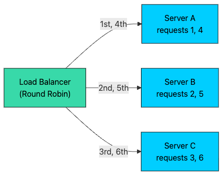
The load balancer only needs a pointer to the next server in the list, which it advances after every request.

servers = [A, B, C]
next = 0

on request:
    server = servers[next]
    next = (next + 1) % len(servers)
    forward request to server

The biggest advantage of round robin is its simplicity. The load balancer doesn’t need to track how busy each server is. It only needs to know which servers are healthy, so it can skip the ones that fail their health checks.

That’s why round robin is the default in many load balancers, including NGINX and HAProxy. For a fleet of identical servers handling short, similar requests, it’s usually good enough.

Round robin assumes all servers are equally capable. In real systems, that’s not always true.

For example, Server A might have sixteen CPU cores while Server B has only four. Round robin would still send both servers the same amount of traffic, even though Server A can handle far more. Server B fills up while Server A sits half idle.

To account for differences in server capacity, we can consider the next algorithm.

Share

Weighted round robin works like regular round robin, except each server is assigned a weight based on its capacity, such as CPU, memory, or overall processing power. The load balancer distributes requests in proportion to those weights.

Suppose the weights are A = 4, B = 2, and C = 1. Out of every seven requests, four go to A, two go to B, and one goes to C.

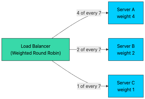
Here, Server A receives roughly four times as much traffic as Server C, which matches the difference in their capacity.

Weighted round robin considers how much traffic each server should receive, not how busy that server actually is right now.

Say Server A receives a few slow, long-running requests and becomes heavily loaded. Weighted round robin doesn’t know that. It keeps sending A four out of every seven requests, simply because of its assigned weight.

To handle this better, the load balancer needs to look at what’s happening on the servers. The simplest signal is the number of active connections each server is handling.

With least connections, the load balancer keeps track of how many active connections each server is currently handling. The next request is sent to the server with the fewest active connections.

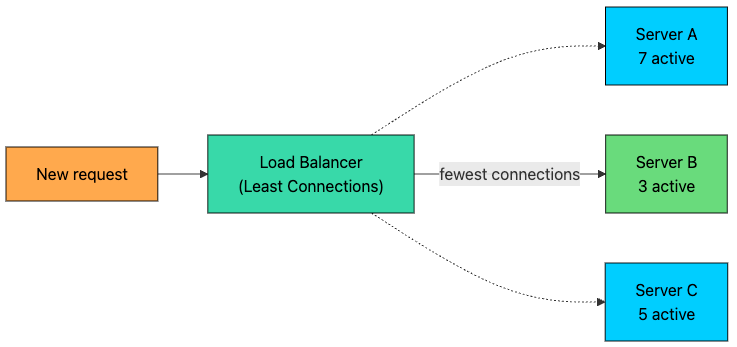
Server B has 3 active connections, the fewest of the three, so the new request goes to B. When a connection closes, the load balancer decrements that server’s count.

This works well when requests or connections can last for very different amounts of time.

Take WebSockets. One connection might stay open for a few seconds while another stays active for several minutes or hours. Round robin would keep handing new connections to a server that’s already holding hundreds of long-lived ones. Least connections adapts by sending new requests only to servers handling fewer connections.

The same applies to any workload with a wide spread of request durations: file uploads, streaming responses, long-polling, or API calls that sometimes take seconds and sometimes take milliseconds.

Connection counts ignore server capacity. Five connections on a small server might be more demanding than ten connections on a much more powerful one. Least connections only sees five versus ten, so it sends the next request to the small server, which is the one that’s already struggling.

So the next algorithm combines connection count with server capacity.

Weighted least connections considers two things at the same time: how busy a server is and how much capacity it has.

Each server gets a weight, just like in weighted round robin. The load balancer then compares servers by the ratio of active connections to weight, and picks the server with the lowest ratio.

on request:
    best = server with minimum (active_connections / weight)
    forward request to best

If Server A is twice as powerful as Server B, it should be able to handle twice as many active connections before we consider it equally loaded.

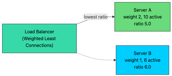
Server A has more raw connections (10 versus 6), but relative to its capacity it’s less loaded, so it gets the request.

Connection count is still only an approximation of actual load. Two connections can consume very different amounts of resources. One might be mostly idle, waiting on the client. Another might be running an expensive computation or a heavy database query.

A server with three idle connections and a server with three heavy ones look identical to any connection-based algorithm. So instead of looking only at connections, we can measure how quickly each server is actually responding.

With least response time, the load balancer looks at how quickly each server is responding, and routes new requests toward the servers that are responding fastest.

The load balancer measures response time for the requests it forwards, usually as a moving average over a recent window. Many implementations combine this with the active connection count, so a fast server that’s also lightly loaded ranks highest.

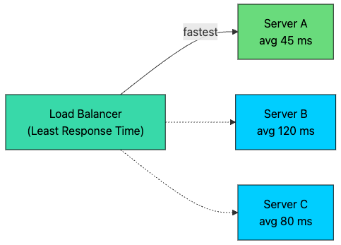
Here, Server A is currently responding the fastest, so it becomes a strong candidate for the next request. The goal is simple: route more traffic toward servers that are performing well right now.

This makes the algorithm more adaptive than round robin or least connections. If a server slows down due to high CPU usage, a garbage collection pause, or a noisy neighbour on the same host, its response times climb. The load balancer notices and temporarily sends it less traffic. When the server recovers, its response times drop and traffic returns.

This flexibility comes with extra complexity. The load balancer has to continuously measure and update server performance, and those measurements can become outdated quickly. This can cause traffic to oscillate between servers.

At very large scale, tracking a fresh, accurate number for every server in the fleet gets expensive. So large systems often use a simpler approach.

With Power of Two Choices, the load balancer doesn’t try to find the least-loaded server across the entire fleet. It randomly picks two servers, compares their current load, and sends the request to the less busy one.

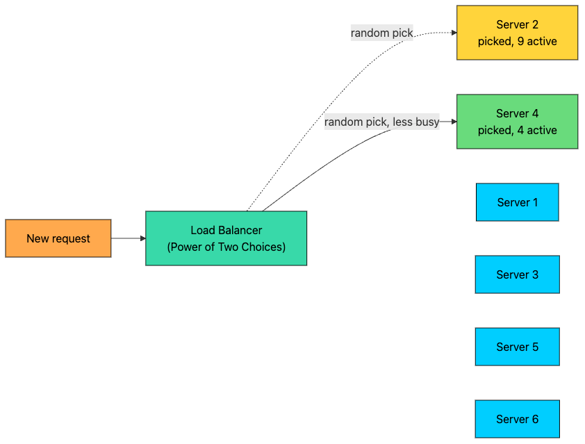
The load balancer sampled servers 2 and 4 at random. Server 4 has fewer active connections, so it wins. The other four servers weren’t examined at all.

on request:
    s1 = random server
    s2 = random server (different from s1)
    forward request to whichever of s1, s2 has lower load

This becomes especially useful at large scale. Suppose you have thousands of backend servers. Finding the least-loaded server across the entire fleet for every request would require a lot of coordination and constantly updated load information for every server.

With Power of Two Choices, each load balancer checks just two servers, and the fleet still ends up with a very good distribution of traffic.

All the algorithms we’ve covered so far assume that any request can go to any healthy server. Sometimes that’s not what we want. We may want requests from the same client to consistently reach the same server.

With IP Hash, the load balancer uses the client’s IP address to decide which server should handle the request. In the simplest version, it hashes the client’s IP address and takes the result modulo the number of servers. That gives the server index.

on request:
    index = hash(client_ip) % number_of_servers
    forward request to servers[index]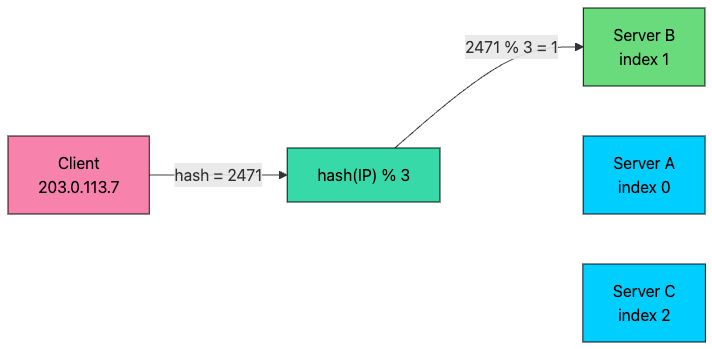

The hash of this client’s address is 2471. Modulo three, that’s 1, so every request from this client lands on Server B. So long as the same client keeps sending requests from the same IP address, those requests will usually go to the same server.

This is useful when you want session affinity, also called sticky sessions.

Suppose a user logs in and some session data is stored locally on Server B, in memory or on local disk. With IP Hash, future requests from that user keep going back to Server B, so the server can reuse that local session data. Without stickiness, the next request might land on Server A, which has never heard of this user and forces a fresh login.

Suppose we have four servers and calculate hash(IP) % 4. Now we add a fifth server, and the calculation changes to hash(IP) % 5.

Most of the clients now map to a different server. In general, changing the modulus from N to N+1 remaps roughly N/(N+1) of all keys, so with four servers about 80% of clients move.

That means most sessions break at once. It can be especially painful for distributed caches or stateful systems, where we want mappings to remain stable as servers are added or removed.

To solve that problem, we can use consistent hashing.

With consistent hashing, we still use hashing to decide where requests should go, but we avoid the biggest problem of remapping with simple modulo hashing.

The idea is to place both servers and keys on a logical hash ring. Each server is hashed onto a position on the ring. When a request comes in, we hash its key (the client IP, a user ID, a cache key), place that key on the ring, and then walk clockwise to the next server on the ring. That server owns the key.

Here is what the ring looks like with three servers and a handful of keys. Each key belongs to the first server it meets walking clockwise.

Keys 42 and 60 walk clockwise and hit Server B first, so B owns them. Key 150 lands on C. Key 340 wraps around the end of the ring and lands on A.

When the server list changes, only the keys near the affected server need to move.

Add a new Server D at position 200. It takes over the keys between B (90) and 200, which used to belong to C. Every other key stays exactly where it was. Remove Server B, and only B’s keys move, to the next server clockwise. Nothing else on the ring notices.

Compare that with modulo hashing, where adding one server remapped around 80% of the keys. With consistent hashing, adding one server to N remaps about 1/(N+1) of the keys, the minimum possible.

That makes consistent hashing especially useful for systems like distributed caches, databases, and storage systems, where moving too many keys at once can be expensive. Memcached clients, Amazon’s DynamoDB, Apache Cassandra, and most CDNs rely on some form of it.

There is one more practical detail. If each physical server appears only once on the ring, the distribution can become uneven. Three servers hashed to random positions might end up owning 25%, 17%, and 58% of the ring. The unlucky server takes more than half the traffic.

So real systems use virtual nodes. Instead of placing each server on the ring once, we place it at many different positions, say 100 or more, each under a different hash such as hash("A-1"), hash("A-2"), and so on.

A few rules of thumb:

• Start with round robin or weighted round robin if your requests are short and similar. Most stateless web APIs never need more.

• Switch to least connections (weighted if the hardware differs) when connections are long-lived or request durations vary a lot.

• Use Power of Two Choices when the fleet is large or when several load balancers share the same backends. It avoids the herd effect of everyone chasing the same “least loaded” server.

• Reach for IP Hash or consistent hashing only when requests genuinely need to land on a specific server. If you can move session state into a shared store like Redis, do that instead, and keep the freedom to send any request anywhere.

• Prefer consistent hashing over plain IP Hash whenever the server list changes with any regularity, which in an autoscaled environment is always.

A load balancer may seem like a small part of the system, but it has a big impact on how the system behaves under heavy traffic.

The key is understanding what each algorithm pays attention to, what it ignores, and when those trade-offs matter.

Thank you for reading!

If you found it valuable, hit a like ❤️ and consider subscribing for more such content every week.

If you have any questions/suggestions, feel free to leave a comment