









Some time ago I started implementing “classic” packet radio into PacketRF. Not the fancy NPR stuff, not high-speed links, but the old and simple AX.25. The one that runs at 1200 baud over a narrow FM channel and somehow still works over surprisingly long distances.
And as soon as I decided to support 1200 baud packet radio (often called PR1200) in PacketRF, I ran into a problem that many people before me had already solved, but I had never really thought about in detail: how do you efficiently decode Bell 202 AFSK on a small embedded system without wasting half your CPU on it?
This post is a write-up of what I learned. Part refresher, part rediscovery, part “wait, why does this even work?”. I ended up making a bunch of small visualizations along the way, mostly out of curiosity, and at some point I realized this is actually a very nice way to look at DFT and Goertzel that I personally had never seen presented this way.
So this is not a textbook explanation. This is more like: I needed this for PacketRF, I looked into it, and this is what finally made it understandable for me. And I also wanted to share my fancy animated GIFs :)
Let’s start from the beginning. Packet radio is one of those things that “everyone knows”, but if you ask three people what PR actually is, you will probably get three slightly different answers.
Classic packet radio (on VHF/UHF) is basically a stack of very simple building blocks layered on top of each other:
And specifically for 1200 baud, this is Bell 202, which uses two tones:
So the whole chain looks like this:
TX:  HDLC frames → NRZI → bits → AFSK (1200/2200 Hz) → audio → radio
RX:  radio → audio → detect tones → bits → NRZI decode → HDLC frames
The part we care about in this article is just one small piece of that chain: detect tones and turn them into bits in the receiver path. So the question we will be solving in the rest of this text is:
Given a chunk of audio samples, how do we decide whether it contains 1200 Hz or 2200 Hz?
That’s it. That’s the entire problem.
If you have ever seen anything about signal processing, you are probably already thinking: “just run an FFT and look at the bins”. And yes, that would work perfectly fine. Take a window of samples, run FFT, check the bins around 1200 Hz and 2200 Hz, compare energies, done. Except… we are not doing this on a desktop CPU, but on a small MCU, something in the “few hundred MHz, limited RAM, lots of other tasks and interupts happening at the same time” category. And a full FFT means:
For AFSK, we only need two frequencies. Everything else is wasted work. So naturally the question becomes: can we compute just those two frequencies directly, without doing a full FFT?
There is a classic trick for exactly this situation called Goertzel algorithm. If you google it, you will almost immediately find something like:
and then second expression for the final result:
At which point everything is, of course, completely obvious and we can all go home and implement it in C++.
Or… not really. Because if someone drops those equations on you without context, you don’t actually understand anything. You just copy them into code and hope for the best. At least that would have been me. I did have signal processing at university, but that was a long time ago, and Goertzel either wasn’t there or I successfully forgot it. So I ended up doing what I usually do in these situations: derive it from something I understand, and build intuition from there. And that “something” is DFT.
Before Goertzel, there is the discrete Fourier transform, usually written like this:
Yes, it looks scary, but the idea behind it is actually very simple if you ignore the notation for a moment. DFT takes your signal and asks: “How much of frequency is present in this signal?”.
Where each frequency corresponds to a bin:
So if we are sampling at 48 kHz and we care about 2200 Hz, then the bin index is roughly:
The interesting part is not the formula itself, but what it means. Look at this term:
This is just a point rotating on the unit circle in the complex plane.
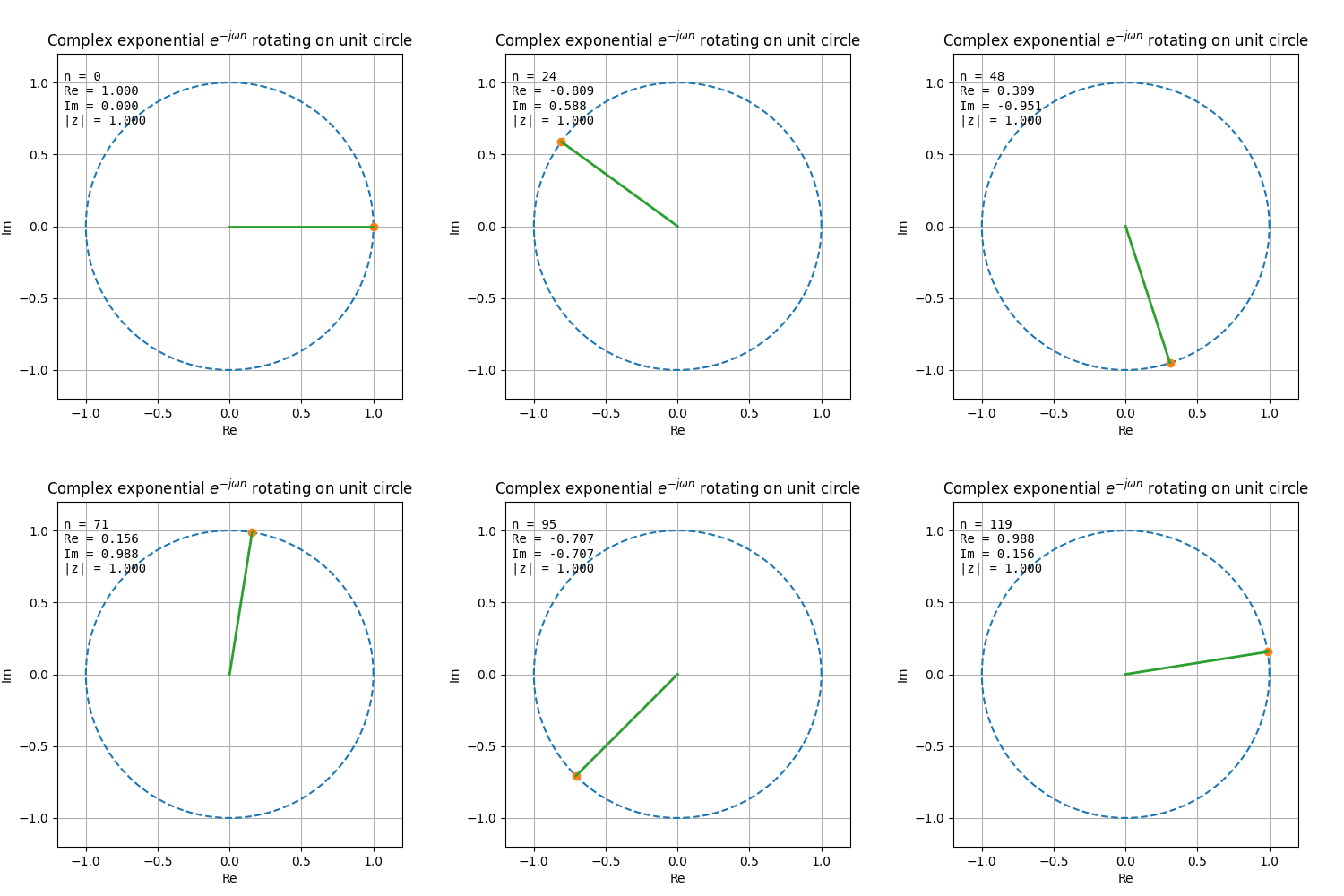
Every sample :
Now look at the full expression:
At each step we:
So we are essentially projecting the signal onto a rotating reference and accumulating the result. And then something quite interesting happens:
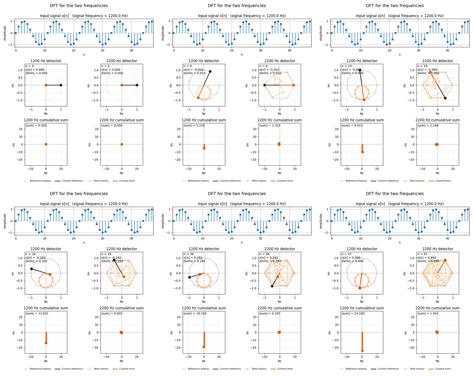
That’s it. That’s the whole magic of DFT. If you stare at the animation above long enough, you can literally see this happening:
For Bell 202, we only care about two frequencies 1200 Hz and 2200 Hz. So what we are really doing is not “FFT” in general, but just computing two DFT bins. The naive way would still require computing sin/cos (or exponentials), complex multiplication and accumulation. Which is still more work than we would like on a small MCU. So the question becomes:
Can we compute the same thing, but in a cheaper way?
Goertzel does not change what we compute. It computes exactly the same DFT bin, but it rewrites the computation into a completely different form. Look at the Goertzel sequence again:
You can probably see, there are no complex numbers, no rotation, just a tiny recursive system.
At this point, when I first saw it written like this, it felt like we jumped from “rotating vectors in complex plane” to “random recursive something” with no explanation in between. On the second look, I could recognize 2nd order IIR filter or a biquad filter.
But how does it help with our AFSK/Bell202 problem? There is an explanation and it turns out to be the most interesting part. At least for me, hopefully for you, too.
Instead of asking “How much of this frequency is in the signal?” we can ask “What happens if I build a tiny oscillator tuned to that frequency, and feed the signal into it?”
Ignore the input for a moment:
This is a second-order system and they tend to oscillate. So what happens if we “tap” it once?
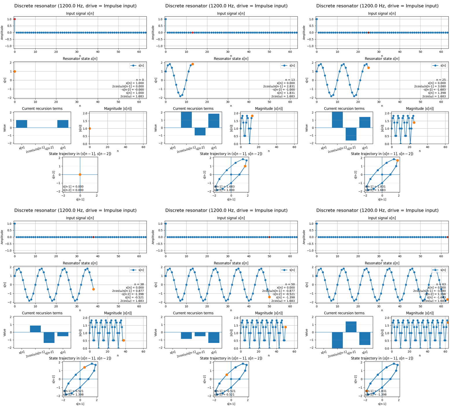
You hit it with a single impulse, and it just keeps oscillating forever. Because this is ideal, mathematically pure oscillator, we have no damping or losses, so it’ll keep oscillating forever. But why it oscillates, you may ask. Let’s look at the math.
If we assume:
and substitute it into the recurrence, everything cancels out nicely and we get the same function back. Which basically proves that the system is perfectly happy oscillating at frequency . This is the discrete equivalent of:
which is just a mass on a spring, or an LC circuit, or any undamped resonator. So this thing is literally a digital spring. Now we bring back the input:
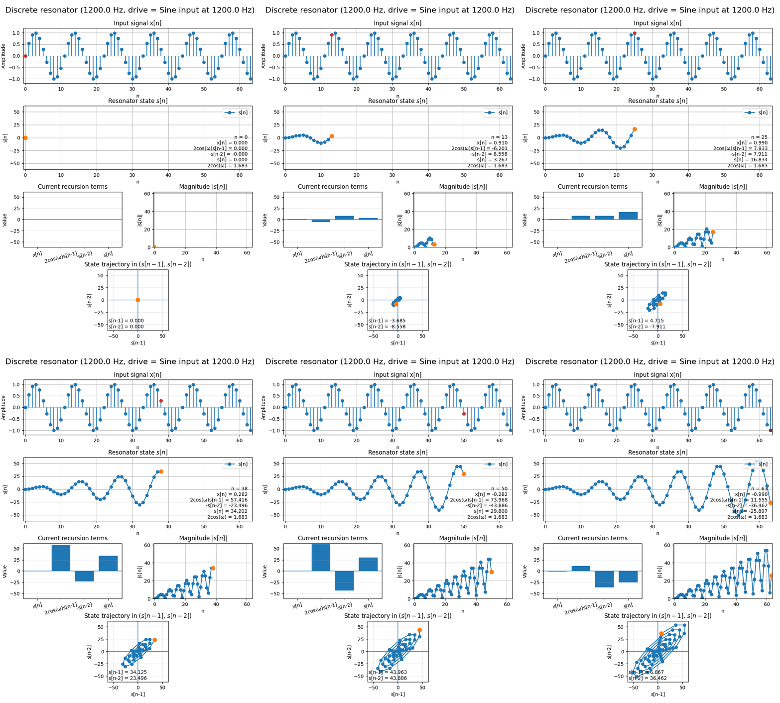
If the input frequency matches the resonator:
If it does not match:
This is exactly the same phenomenon we saw in the DFT view. Just from a completely different angle.
I made this plot where I take one input signal and feed it into multiple resonators tuned to different frequencies.
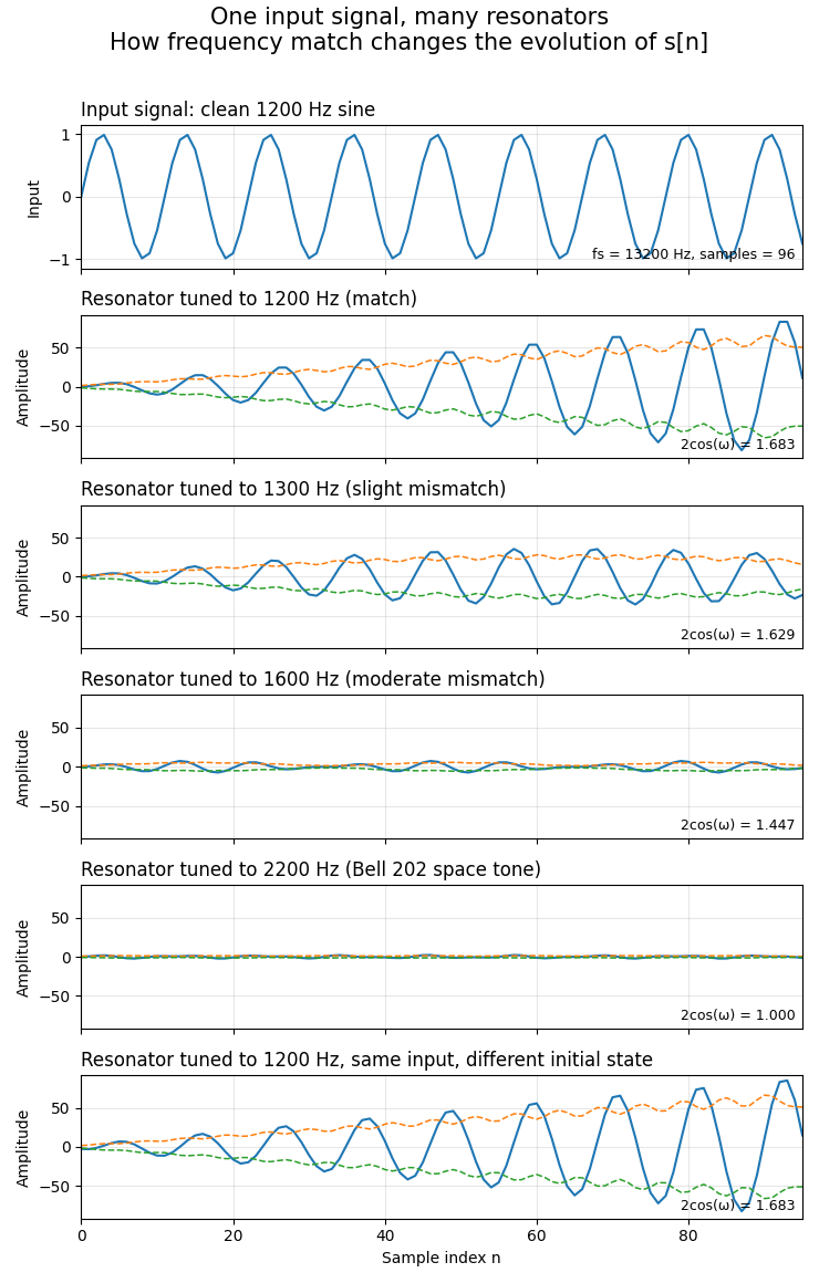
And this is where you can clearly see:
What is that mysterious ? This parameter looks like black magic at first, but it’s actually very simple:
It just encodes the frequency we care about. It determines how the internal state evolves, or if you prefer a more visual description, how the system “rotates” in its own internal space. And the nice thing is:
This was another thing that confused me at first. In the DFT, we explicitly sum complex values. Here we don’t, but the accumulation is still happening. It is just hidden inside the state variables:
At the end of a block of samples, we extract the result like this:
Which is exactly the same energy we would get from the DFT, just without ever computing complex numbers.
At this point, we have everything we need, let’s implement it in the C.
We have seen the DFT view with rotating vectors, we have reinterpreted the same process as a resonator, and we have convinced ourselves that the system accumulates energy when the input frequency matches the one we are looking for. Now comes the slightly anticlimactic moment: the actual implementation. Because once you understand what is going on, the code itself is simple.
Here is a minimal and complete Goertzel implementation in C, written in a way that maps directly to the recurrence we derived:
#include <math.h>
#include <stdint.h>

typedef struct {
    float coeff;   // 2*cos(omega)
    float s_prev;  // s[n-1]
    float s_prev2; // s[n-2]
} goertzel_t;

void goertzel_init(goertzel_t *g, float target_freq, float sample_rate)
{
    float omega = 2.0f * M_PI * target_freq / sample_rate;
    g->coeff = 2.0f * cosf(omega);
    g->s_prev = 0.0f;
    g->s_prev2 = 0.0f;
}

void goertzel_reset(goertzel_t *g)
{
    g->s_prev = 0.0f;
    g->s_prev2 = 0.0f;
}

void goertzel_process_sample(goertzel_t *g, float x)
{
    float s = x + g->coeff * g->s_prev - g->s_prev2;
    g->s_prev2 = g->s_prev;
    g->s_prev = s;
}

float goertzel_get_power(goertzel_t *g)
{
    // |X_k|^2 without explicitly computing complex numbers
    return g->s_prev * g->s_prev +
           g->s_prev2 * g->s_prev2 -
           g->coeff * g->s_prev * g->s_prev2;
}
Initialization:
float omega = 2π f / f_s;
coeff = 2 cos(omega);
This is where we “tune” the resonator to a specific frequency.
If you want to detect two frequencies, you will need two instances of this resonator and that becomes your entire AFSK demodulator.
Processing one sample:
s = x + coeff * s_prev - s_prev2;
This is the recurrence relation we derived earlier.
Every input sample does three things:
x)coeff * s_prev)-s_prev2)Getting the result:
power = s_prev² + s_prev2² - coeff * s_prev * s_prev2;
This is the part that looks slightly magical if you have not seen it before, but it is simply the algebraic way of computing:
without ever touching the complex number. This is the energy at the target frequency over the whole window.
Af we mentioned before, for AFSK Bell 202, we run two of these detectors in parallel:
For each bit window:
bit = (power_1200 >= power_2200) ? 1 : 0;
Now let us connect all of this to something tangible. Here is a real WAV recording of a 1200 baud AFSK packet carrying a simple message:
And here is what the decoder produces:
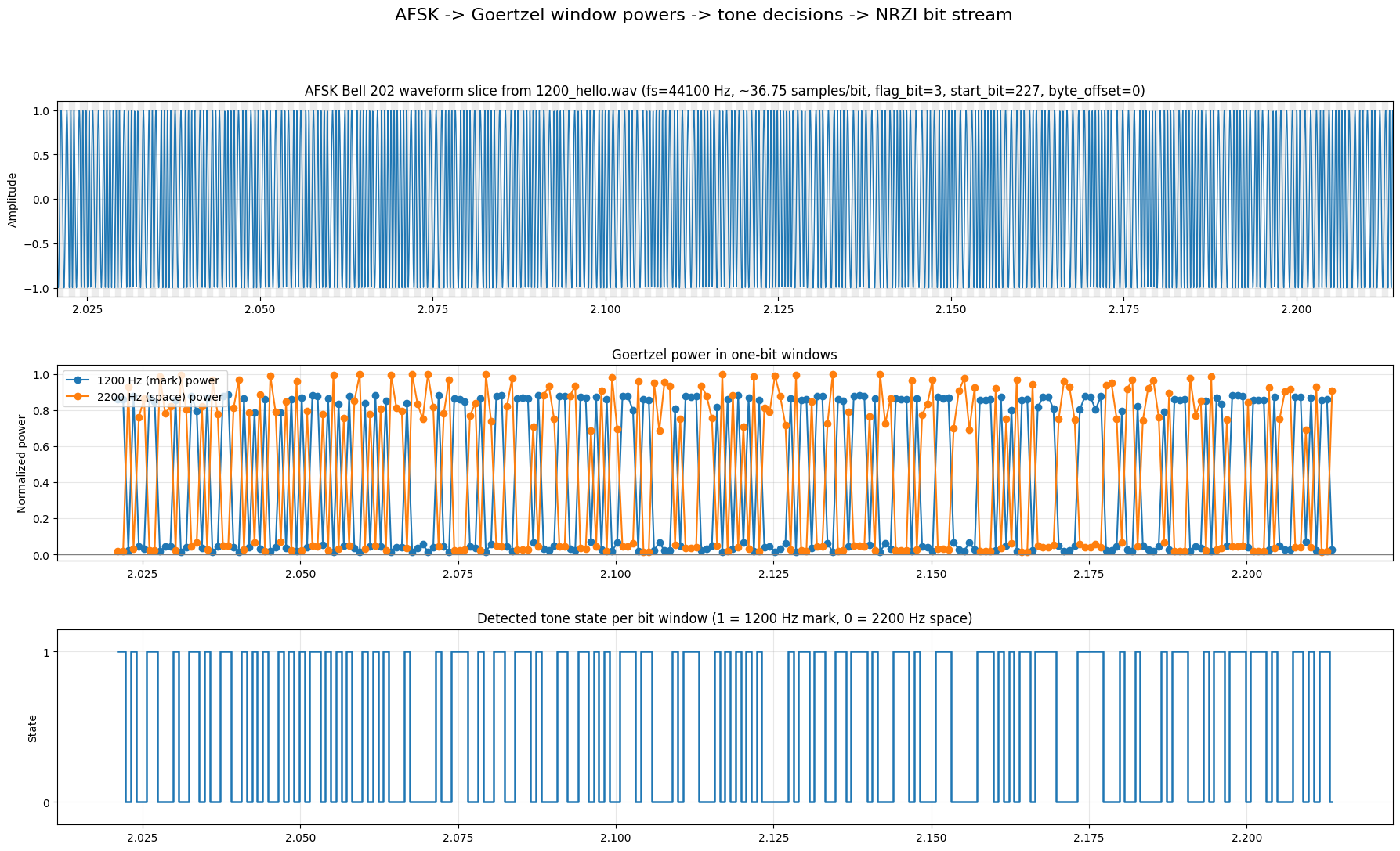
Let us go through the output step by step.
Tone-state stream on wire (232 symbols):
11010011 00010011 01001100 10101001 01010110 10101001 01010001 00000100
11100100 11001110 10001100 11010100 11101100 00101110 00101010 10100000
10110110 01101110 10001110 10001110 00001110 10101101 11100001 11110001
00100001 01110001 01101110 11101000 11010110
This is the raw output of the Goertzel detectors.
At this point:
This is still not bits, only tones.
After NRZI decode:
01000101 01100101 00010101 00000010 00000010 00000010 00000110 01111001
01101001 01010110 00110101 01000001 01100101 11000110 11000000 00001111
00010010 10100110 00110110 00110110 11110110 00000100 11101110 11110110
01001110 00110110 00100110 01100011 01000010
NRZI means:
So we convert tone changes into bits and we finally have a bitstream.
NRZI-decoded bytes (LSB-first):
A2 A6 A8 40 40 40 60 9E 96 6A AC 82 A6 63 03 F0 48 65 6C 6C 6F 20 77 6F 72 6C 64 C6 42
Important detail: AX.25 sends bits least significant bit first. So even though we write bytes in hex, the bit order inside each byte is reversed compared to “normal” binary.
HDLC inserts a 0 after five consecutive 1s. We remove it:
After HDLC bit unstuff:
A2 A6 A8 40 40 40 60 9E 96 6A AC 82 A6 63 03 F0 48 65 6C 6C 6F 20 77 6F 72 6C 64 C6 42
In this particular frame, unstuffing does not change anything, but in general it is required.
A2 A6 A8 40 40 40 60
9E 96 6A AC 82 A6 63
03 F0
48 65 6C 6C 6F 20 77 6F 72 6C 64
C6 42
Now we are looking at a full AX.25 frame.
Let us decode it field by field.
| Bytes | Meaning |
|---|---|
A2 A6 A8 40 40 40 60 | Destination callsign |
9E 96 6A AC 82 A6 63 | Source callsign |
03 | Control field (UI frame) |
F0 | Protocol ID (no layer 3) |
48 65 6C 6C 6F 20 77 6F 72 6C 64 | Payload |
C6 42 | FCS (CRC) |
AX.25 encodes callsigns in a slightly unusual way:
So A2 A6 A8 40 40 40 60 decodes to something like QST 0 and 9E 96 6A AC 82 A6 63 decodes to OK5VAS1.
Actual payload is 48 65 6C 6C 6F 20 77 6F 72 6C 64, which is simply ASCII string Hello world
Last two bytes is CRC C6 42, or sometimes called “Frame Check Sequence”. If you run CRC-16 (X.25) over the frame, you will get this value, which confirms the decode is correct.
At the beginning of this article, we had:
Now, after:
we end up with Hello world message from the audio signal. And the entire chain, from floating-point math down to ASCII text, is visible, understandable, and implementable on a small microcontroller. We could optimize this further for embedded use, including fixed-point arithmetic and running the whole decoder in real time on RP2350, but that’s out of this article scope. If you are curious, look at the source code of the PacketRF.
此内容由惯性聚合(RSS阅读器)自动聚合整理,仅供阅读参考。 原文来自 — 版权归原作者所有。