推荐订阅源

 

 

1.     

[Measures].[Sales Sum] / [Measures].[Item Count]

If you need to take a simple average of values associated with a set of cells,

you can use the MDX Avg() function, as in the following example:

WITH

SET [My States] AS

‘{ [Customer].[MA], [Customer].[ME], [Customer].[MI], [Customer].[MO] }’

MEMBER [Customer].[Avg Over States] AS ‘Avg ([My States])’

SELECT

{ [Measures].[Dollar Sales], [Measures].[Unit Sales] } on columns,

{ [Products].[Family].Members } on rows

FROM Sales

WHERE ([Customer].[Avg Over States])

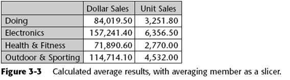
This query returns a grid of three measures by N product families. The sales, units, and profit measures are each averaged over the five best customers in terms of total profit. Notice that the expression to be averaged by the Avg() function has been left unspecified in the [Avg Over States] calculation. Leaving it unspecified is the equivalent of saying:

([Measures].CurrentMember, [Products].CurrentMember , . . . )

 

2.     

Sum (

CrossJoin(

Descendants ([Industry].CurrentMember, [Industry].[Company],

SELF),

Descendants ([Time].CurrentMember, [Time].[Day], SELF)

)

,([Measures].[Share Price] * [Measures].[Units Sold])

) / [Measures].[Units Sold]

will calculate this weighted average.

A difficulty lurks in formulating the query this way, however. The greater the number of dimensions you are including in the average, the larger the size of the cross-joined set. You can run into performance problems (as well as intelligibility problems) if the number of dimensions being combined is large and the server actually builds the cross-joined set in memory while executing this. Moreover, you should account for all dimensions in the cube or you may accidentally involve aggregate [Share Price] values in a multiplication, which will probably be an error. In Analysis Services 2005, you can improve this by using NonEmpty() around a cross-join, as follows:

NonEmpty (

{ [Measures].[Share Price], [Measures].[Units Sold])}

* Descendants ([Industry].CurrentMember,

[Industry].[Company], SELF)

* Descendants ([Time].CurrentMember, [Time].[Day], SELF)

* Descendants ([Customer].CurrentMember, [Time].[Day], SELF))

)

3.    同比（时间）

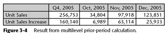
The following is equally valid, and its results are shown in Figure 3-4. Note that the Q4 difference is based on Q3 and Q4 expenses, whereas each month’s difference is based on its expenses and the prior month’s expenses.

WITH MEMBER [Measures].[Unit Sales Increase] AS

‘[Measures].[Unit Sales]

- ([Measures].[Unit Sales], [Time].CurrentMember.PrevMember)’

SELECT

{ [Time].[Q4, 2005], [Time].[Q4, 2005].Children } on columns,

{ [Measures].[Unit Sales], [Measures].[Unit Sales Increase] }

on rows

FROM Sales

 

4.    环比

PeriodsToDate ( [Time].[Year], [Time].CurrentMember ),

[Measures].[Dollar Sales]

)’

SELECT

{ [Time].[Quarter].[Q3, 2000], [Time].[Quarter].[Q4, 2000],

[Time].[Quarter].[Q1, 2001]

} on columns,

{ [Measures].[Expenses], [Measures].[YTD Expenses] } on rows

FROM Costing

Note that the [Unit Sales YAgo Increase] for Q1, 2005 is the difference

in first-quarter sales, whereas the [Unit Sales YAgo Increase] for Jan,

2005 is the difference in January sales.

5.    Year-to-Date (Period-to-Date) Aggregations

WITH MEMBER [Measures].[YTD Dollar Sales] AS

‘Sum (

PeriodsToDate ( [Time].[Year], [Time].CurrentMember ),

[Measures].[Dollar Sales]

)’

SELECT

{ [Time].[Quarter].[Q3, 2000], [Time].[Quarter].[Q4, 2000],

[Time].[Quarter].[Q1, 2001]

} on columns,

{ [Measures].[Expenses], [Measures].[YTD Expenses] } on rows

FROM Costing

If the time dimension is tagged as being of Time type and the year level within it is tagged as being of type Year, then you could also use the shorthand:

‘Sum (

YTD ([Time].CurrentMember),

[Measures].[Expenses]

)’

or even:

‘Sum (

YTD (),

[Measures].[Expenses]

)

6.     

For example, the following returns

all months from the first month in the time dimension to July, 2005:

{ NULL : [Time].[Jul, 2005] }

In a more standard way, you can reference the first member at the current level of the time dimension with one of the following expressions:

[Time].CurrentMember.Level.Members.Item(0)

OpeningPeriod ([Time].[All Time], [Time].CurrentMember.Level)

OpeningPeriod ([Time], [Time].CurrentMember.Level) The first way takes the level of the current time member, gets its members, and selects the first member in it, whereas the second one simply asks for the opening period at the current member’s level across all times.

The second way also requires an All level in the time dimension, which may or may not be defined. Using the second approach, you could specify:

WITH MEMBER [Measures].[All Accumulated Unit Sales] AS

‘Sum (

{ OpeningPeriod ([Time].CurrentMember.Level, [Time].[All Time])

: [Time].CurrentMember },

[Measures].[Expenses]

)’

SELECT

{ [Time].[Quarter].[Q3, 2005], [Time].[Quarter].[Q4, 2005]

} on columns,

{ [Measures].[Unit Sales], [Measures].[All Accumulated Unit Sales] } on

rows

FROM Sales

The most direct way, if the time dimension has an All level, is simply to use

PeriodsToDate() with the [Time].[(All)] level:

WITH MEMBER [Measures].[All Accumulated Expenses] AS

‘Sum (

PeriodsToDate ( [Time].[(All)], [Time].CurrentMember ),

[Measures].[Expenses]

)’

SELECT

...

7.     

in Analysis Services 2005, attribute members are tightly linked to base dimension members, so that the current member of the base dimension influences the current member of the attribute member. So we could filter product SKUs by their ship weight with the following as well:

Filter (

[Product].[ByCategory].[SKU].Members,

[Product].[ShipWeight].CurrentMember.MemberValue

>= 1

AND

[Product].[ShipWeight].CurrentMember.MemberValue

<= 5

)

Remember that member properties are defined for a particular level, but when you reference them through the .Properties() function, only the name is of interest, not the unique name. This means that if the same property name is in two or more levels, all of them will return a result when referenced through the .Properties() function. In the case of parent-child dimensions, a member property is defined for every apparent level (except perhaps the All level, depending on the dimension definition), because internally, all parent-child members are stored in one database level. Every query passes through five main execution stages after the query is successfully parsed. The stages, in order, are

1. Resolving the FROM clause (if any—it is optional in Essbase)

2. Resolving the WHERE clause, if any

3. Resolving named sets in the WITH clause

4. Resolving the tuples on each axis

5. Calculating the cells brought back in the axis intersections

a. Resolving NON EMPTY intersections

b. (AS2005) Resolving the HAVING clause on each axis

Physically, there is no requirement that this is the required order, but logically

this is the sequence. Figure 4-1 provides a conceptual flowchart of the

process.

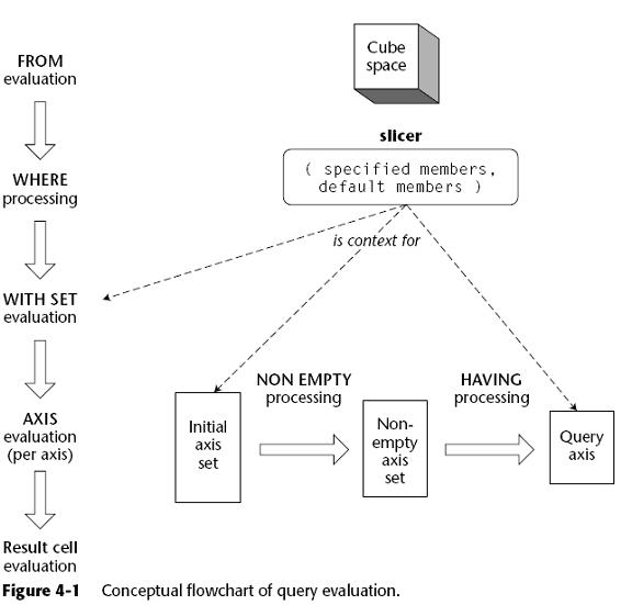
Along the way, there is always a default cell context and a default iteration context. This starts from outside the query and is always carried from one stage to the next. Each stage can modify this context before passing on to the next stage.

8.     

SELECT

{[Product].[Health], [Product].[Shaving]}

on axis(0)

FROM [Sales]

WHERE ([Time].[2005], [Measures].[Dollar Sales])

After the slicer is evaluated, the cell context used in evaluating the product

members is still:

( Time.[2005],

Product.DefaultMember,

Customer.DefaultMember,

Promotion.DefaultMember,

Measures.[Dollar Sales]

)’

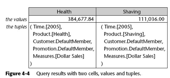
Because the axis is defined by enumerating member names, it doesn’t matter what the cell context is. Once the axis is resolved, the cell data can be pulled back. The two tuples effectively pulled back are shown in Figure 4-4.

 

9.     

SELECT

Filter (

[Product].[Category].Members,

[Measures].[Dollars Sold] > 900000

)

on axis(0)

FROM Sales

WHERE ([Time].[2005], [Measures].[Dollars Sold])

The cell context after the WHERE clause is resolved as before. This means that when the Filter() is executing, the values associated with the members are as follows.

The data values that are compared to 900,000 are from the tuples shown in Figure 4-5. Note that the cell context set up by the slicer is passed along during the evaluation of the axis. Once the filter has returned a set of members, the axis is resolved and you will see the results, as shown in Figure 4-6.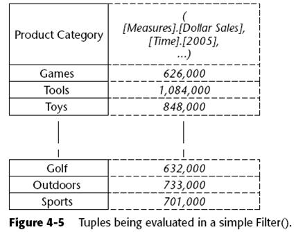

Within the Filter(), you can take this context tuple and modify it. Consider the following query, which filters the product categories where Dollar Sales increased more than 40 percent from the previous year:

SELECT

Filter (

[Product].[Category].Members,

[Measures].[Dollar Sales] >

1.4 *

( [Measures].[Dollar Sales],

[Time].CurrentMember.PrevMember )

)

on axis(0)

FROM Sales

WHERE ([Time].[2005], [Measures].[Dollar Sales])

The slicer sets up ([Time].[2005], [Measures].[Dollar Sales])

again. Within the filter, the Dollar Sales are compared to the Dollar Sales from

the previous time member. As the time component of the context is [2005],the previous time member will be 2004. Inside this filter, the comparisons made are shown in Figure 4-7.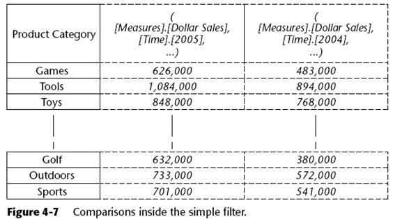

Because the context carries one member from each dimension in it, you can rely even more on it in your expressions. Aquery that performs the same work as the previous query, but phrased in a different way, is as follows:

SELECT

Filter (

[Product].[Category].Members,

[Time].CurrentMember >

1.4 * [Time].CurrentMember.PrevMember

)

on axis(0)

FROM Sales

WHERE ([Time].[2005], [Measures].[Dollar Sales])

The Filter()’s comparison expression doesn’t refer to any fixed points at all. Because the context of the Filter() includes [Measures].[Dollar

Sales], that is what is used. You would choose to build a query this way if you only wanted to specify the measure in one place. Looking at this as an example of a Filter() expression more than as a complete query, you also might use it against multiple measures without needing to edit it.

10.             

Just because the slicer provides context doesn’t mean you need to use it. Consider the following query with important portions underlined, and whose results are in Figure 4-8:

SELECT

{ Filter (

[Product].[Category].Members,

([Measures].[Unit Sales], [Time].[Q4, 2005])

> 1.4 * ([Measures].[Unit Sales],

[Time].[Q4, 2004] )

) }

on axis(0)

FROM Sales

WHERE ([Time].[2005], [Measures].[Dollar Sales])

The slicer sets up ([Time].[2005] and [Measures].[Dollar Sales]),

but the Filter() expression compares [Measures].[Unit Sales] at

[Time].[Q4, 2005] and [Time].[Q4, 2004]. The expressions used in the

Filter(), or in any other part of deciding an axis, can selectively rely on or override any portion of the cell context. So the results are Dollar Sales in 2005, but the filter condition was entirely on Unit Sales from other time periods. Although we have been highlighting the columns axis, the following is true for all axes:

■■ Evaluation of each axis takes a cell context from the WHERE clause.

■■ Each axis evaluates independently from the others (except in Analysis

Services when influenced by the Axis() function).

Resolving each axis can involve the computation of an arbitrary number of cells, depending on the expressions involved. Once the axes are resolved, each cell that is retrieved is identified by the tuple formed by combining each axis’ tuple for that cell with the slicer. Any

dimension not explicitly mapped to a tuple has its default member in the slicer.