Back to Articles

This article is also available in Chinese 简体中文.

In this post, you'll learn to build an image similarity system with 🤗 Transformers. Finding out the similarity between a query image and potential candidates is an important use case for information retrieval systems, such as reverse image search, for example. All the system is trying to answer is that, given a query image and a set of candidate images, which images are the most similar to the query image.

We'll leverage the 🤗 datasets library as it seamlessly supports parallel processing which will come in handy when building this system.

Although the post uses a ViT-based model (nateraw/vit-base-beans) and a particular dataset (Beans), it can be extended to use other models supporting vision modality and other image datasets. Some notable models you could try:

• Swin Transformer
• ConvNeXT
• RegNet

Also, the approach presented in the post can potentially be extended to other modalities as well.

To study the fully working image-similarity system, you can refer to the Colab Notebook linked at the beginning.

How do we define similarity?

To build this system, we first need to define how we want to compute the similarity between two images. One widely popular practice is to compute dense representations (embeddings) of the given images and then use the cosine similarity metric to determine how similar the two images are.

For this post, we'll use “embeddings” to represent images in vector space. This gives us a nice way to meaningfully compress the high-dimensional pixel space of images (224 x 224 x 3, for example) to something much lower dimensional (768, for example). The primary advantage of doing this is the reduced computation time in the subsequent steps.

Computing embeddings

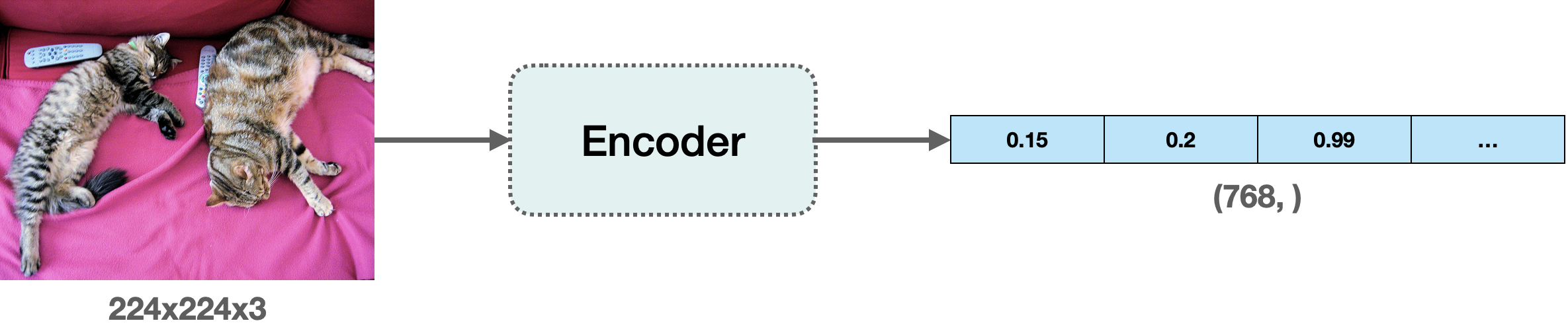
To compute the embeddings from the images, we'll use a vision model that has some understanding of how to represent the input images in the vector space. This type of model is also commonly referred to as image encoder.

For loading the model, we leverage the AutoModel class. It provides an interface for us to load any compatible model checkpoint from the Hugging Face Hub. Alongside the model, we also load the processor associated with the model for data preprocessing.

from transformers import AutoImageProcessor, AutoModel


model_ckpt = "nateraw/vit-base-beans"
processor = AutoImageProcessor.from_pretrained(model_ckpt)
model = AutoModel.from_pretrained(model_ckpt)

In this case, the checkpoint was obtained by fine-tuning a Vision Transformer based model on the beans dataset.

Some questions that might arise here:

Q1: Why did we not use AutoModelForImageClassification?

This is because we want to obtain dense representations of the images and not discrete categories, which are what AutoModelForImageClassification would have provided.

Q2: Why this checkpoint in particular?

As mentioned earlier, we're using a specific dataset to build the system. So, instead of using a generalist model (like the ones trained on the ImageNet-1k dataset, for example), it's better to use a model that has been fine-tuned on the dataset being used. That way, the underlying model better understands the input images.

Note that you can also use a checkpoint that was obtained through self-supervised pre-training. The checkpoint doesn't necessarily have to come from supervised learning. In fact, if pre-trained well, self-supervised models can yield impressive retrieval performance.

Now that we have a model for computing the embeddings, we need some candidate images to query against.

Loading a dataset for candidate images

In some time, we'll be building hash tables mapping the candidate images to hashes. During the query time, we'll use these hash tables. We'll talk more about hash tables in the respective section but for now, to have a set of candidate images, we will use the train split of the beans dataset.

from datasets import load_dataset


dataset = load_dataset("beans")

This is how a single sample from the training split looks like:

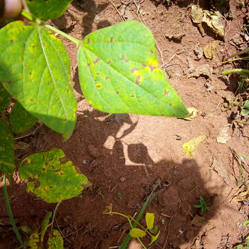
The dataset has three features:

dataset["train"].features
>>> {'image_file_path': Value(dtype='string', id=None),
 'image': Image(decode=True, id=None),
 'labels': ClassLabel(names=['angular_leaf_spot', 'bean_rust', 'healthy'], id=None)}

To demonstrate the image similarity system, we'll use 100 samples from the candidate image dataset to keep the overall runtime short.

num_samples = 100
seed = 42
candidate_subset = dataset["train"].shuffle(seed=seed).select(range(num_samples))

The process of finding similar images

Below, you can find a pictorial overview of the process underlying fetching similar images.

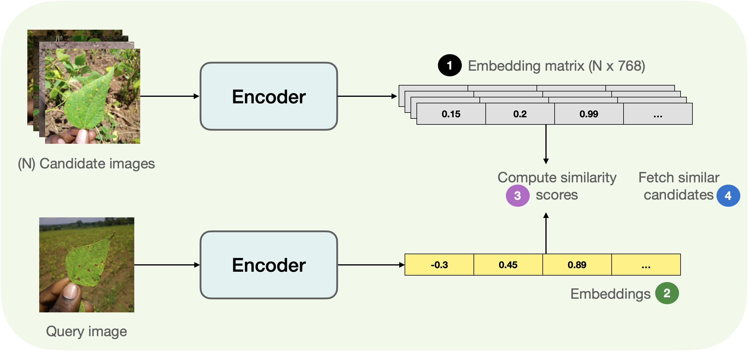
Breaking down the above figure a bit, we have:

1. Extract the embeddings from the candidate images (candidate_subset), storing them in a matrix.
2. Take a query image and extract its embeddings.
3. Iterate over the embedding matrix (computed in step 1) and compute the similarity score between the query embedding and the current candidate embeddings. We usually maintain a dictionary-like mapping maintaining a correspondence between some identifier of the candidate image and the similarity scores.
4. Sort the mapping structure w.r.t the similarity scores and return the underlying identifiers. We use these identifiers to fetch the candidate samples.

We can write a simple utility and map() it to our dataset of candidate images to compute the embeddings efficiently.

import torch 

def extract_embeddings(model: torch.nn.Module):
    """Utility to compute embeddings."""
    device = model.device

    def pp(batch):
        images = batch["image"]
        # `transformation_chain` is a compostion of preprocessing
        # transformations we apply to the input images to prepare them
        # for the model. For more details, check out the accompanying Colab Notebook.
        image_batch_transformed = torch.stack(
            [transformation_chain(image) for image in images]
        )
        new_batch = {"pixel_values": image_batch_transformed.to(device)}
        with torch.no_grad():
            embeddings = model(**new_batch).last_hidden_state[:, 0].cpu()
        return {"embeddings": embeddings}

    return pp

And we can map extract_embeddings() like so:

device = "cuda" if torch.cuda.is_available() else "cpu"
extract_fn = extract_embeddings(model.to(device))
candidate_subset_emb = candidate_subset.map(extract_fn, batched=True, batch_size=batch_size)

Next, for convenience, we create a list containing the identifiers of the candidate images.

candidate_ids = []

for id in tqdm(range(len(candidate_subset_emb))):
    label = candidate_subset_emb[id]["labels"]

    # Create a unique indentifier.
    entry = str(id) + "_" + str(label)

    candidate_ids.append(entry)

We'll use the matrix of the embeddings of all the candidate images for computing the similarity scores with a query image. We have already computed the candidate image embeddings. In the next cell, we just gather them together in a matrix.

all_candidate_embeddings = np.array(candidate_subset_emb["embeddings"])
all_candidate_embeddings = torch.from_numpy(all_candidate_embeddings)

We'll use cosine similarity to compute the similarity score in between two embedding vectors. We'll then use it to fetch similar candidate samples given a query sample.

def compute_scores(emb_one, emb_two):
    """Computes cosine similarity between two vectors."""
    scores = torch.nn.functional.cosine_similarity(emb_one, emb_two)
    return scores.numpy().tolist()


def fetch_similar(image, top_k=5):
    """Fetches the `top_k` similar images with `image` as the query."""
    # Prepare the input query image for embedding computation.
    image_transformed = transformation_chain(image).unsqueeze(0)
    new_batch = {"pixel_values": image_transformed.to(device)}

    # Comute the embedding.
    with torch.no_grad():
        query_embeddings = model(**new_batch).last_hidden_state[:, 0].cpu()

    # Compute similarity scores with all the candidate images at one go.
    # We also create a mapping between the candidate image identifiers
    # and their similarity scores with the query image.
    sim_scores = compute_scores(all_candidate_embeddings, query_embeddings)
    similarity_mapping = dict(zip(candidate_ids, sim_scores))
 
    # Sort the mapping dictionary and return `top_k` candidates.
    similarity_mapping_sorted = dict(
        sorted(similarity_mapping.items(), key=lambda x: x[1], reverse=True)
    )
    id_entries = list(similarity_mapping_sorted.keys())[:top_k]

    ids = list(map(lambda x: int(x.split("_")[0]), id_entries))
    labels = list(map(lambda x: int(x.split("_")[-1]), id_entries))
    return ids, labels

Perform a query

Given all the utilities, we're equipped to do a similarity search. Let's have a query image from the test split of the beans dataset:

test_idx = np.random.choice(len(dataset["test"]))
test_sample = dataset["test"][test_idx]["image"]
test_label = dataset["test"][test_idx]["labels"]

sim_ids, sim_labels = fetch_similar(test_sample)
print(f"Query label: {test_label}")
print(f"Top 5 candidate labels: {sim_labels}")

Leads to:

Query label: 0
Top 5 candidate labels: [0, 0, 0, 0, 0]

Seems like our system got the right set of similar images. When visualized, we'd get:

Further extensions and conclusions

We now have a working image similarity system. But in reality, you'll be dealing with a lot more candidate images. Taking that into consideration, our current procedure has got multiple drawbacks:

• If we store the embeddings as is, the memory requirements can shoot up quickly, especially when dealing with millions of candidate images. The embeddings are 768-d in our case, which can still be relatively high in the large-scale regime.
• Having high-dimensional embeddings have a direct effect on the subsequent computations involved in the retrieval part.

If we can somehow reduce the dimensionality of the embeddings without disturbing their meaning, we can still maintain a good trade-off between speed and retrieval quality. The accompanying Colab Notebook of this post implements and demonstrates utilities for achieving this with random projection and locality-sensitive hashing.

🤗 Datasets offers direct integrations with FAISS which further simplifies the process of building similarity systems. Let's say you've already extracted the embeddings of the candidate images (the beans dataset) and stored them inside a feature called embeddings. You can now easily use the add_faiss_index() of the dataset to build a dense index:

dataset_with_embeddings.add_faiss_index(column="embeddings")

Once the index is built, dataset_with_embeddings can be used to retrieve the nearest examples given query embeddings with get_nearest_examples():

scores, retrieved_examples = dataset_with_embeddings.get_nearest_examples(
    "embeddings", qi_embedding, k=top_k
)

The method returns scores and corresponding candidate examples. To know more, you can check out the official documentation and this notebook.

Finally, you can try out the following Space that builds a mini image similarity application:

In this post, we ran through a quickstart for building image similarity systems. If you found this post interesting, we highly recommend building on top of the concepts we discussed here so you can get more comfortable with the inner workings.

Still looking to learn more? Here are some additional resources that might be useful for you:

• Faiss: A library for efficient similarity search
• ScaNN: Efficient Vector Similarity Search
• Integrating Image Searchers within Mobile Applications