Back to Articles

Unit 2, part 1 of the Deep Reinforcement Learning Class with Hugging Face 🤗

⚠️ A new updated version of this article is available here 👉 https://huggingface.co/deep-rl-course/unit1/introduction

This article is part of the Deep Reinforcement Learning Class. A free course from beginner to expert. Check the syllabus here.

---

⚠️ A new updated version of this article is available here 👉 https://huggingface.co/deep-rl-course/unit1/introduction

This article is part of the Deep Reinforcement Learning Class. A free course from beginner to expert. Check the syllabus here.

In the first chapter of this class, we learned about Reinforcement Learning (RL), the RL process, and the different methods to solve an RL problem. We also trained our first lander agent to land correctly on the Moon 🌕 and uploaded it to the Hugging Face Hub.

So today, we're going to dive deeper into one of the Reinforcement Learning methods: value-based methods and study our first RL algorithm: Q-Learning.

We'll also implement our first RL agent from scratch: a Q-Learning agent and will train it in two environments:

1. Frozen-Lake-v1 (non-slippery version): where our agent will need to go from the starting state (S) to the goal state (G) by walking only on frozen tiles (F) and avoiding holes (H).
2. An autonomous taxi will need to learn to navigate a city to transport its passengers from point A to point B.

This unit is divided into 2 parts:

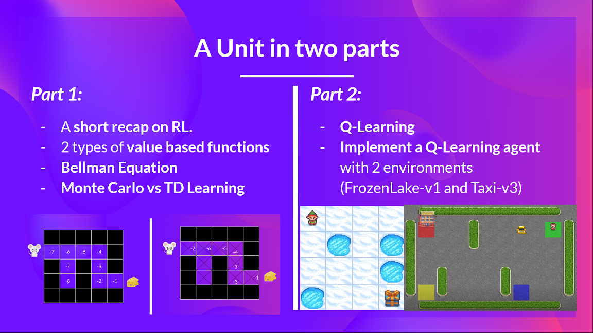
In the first part, we'll learn about the value-based methods and the difference between Monte Carlo and Temporal Difference Learning.

And in the second part, we'll study our first RL algorithm: Q-Learning, and implement our first RL Agent.

This unit is fundamental if you want to be able to work on Deep Q-Learning (unit 3): the first Deep RL algorithm that was able to play Atari games and beat the human level on some of them (breakout, space invaders…).

So let's get started!

• What is RL? A short recap
• The two types of value-based methods
  • The State-Value function
  • The Action-Value function
• The Bellman Equation: simplify our value estimation
• Monte Carlo vs Temporal Difference Learning
  • Monte Carlo: learning at the end of the episode
  • Temporal Difference Learning: learning at each step

What is RL? A short recap

In RL, we build an agent that can make smart decisions. For instance, an agent that learns to play a video game. Or a trading agent that learns to maximize its benefits by making smart decisions on what stocks to buy and when to sell.

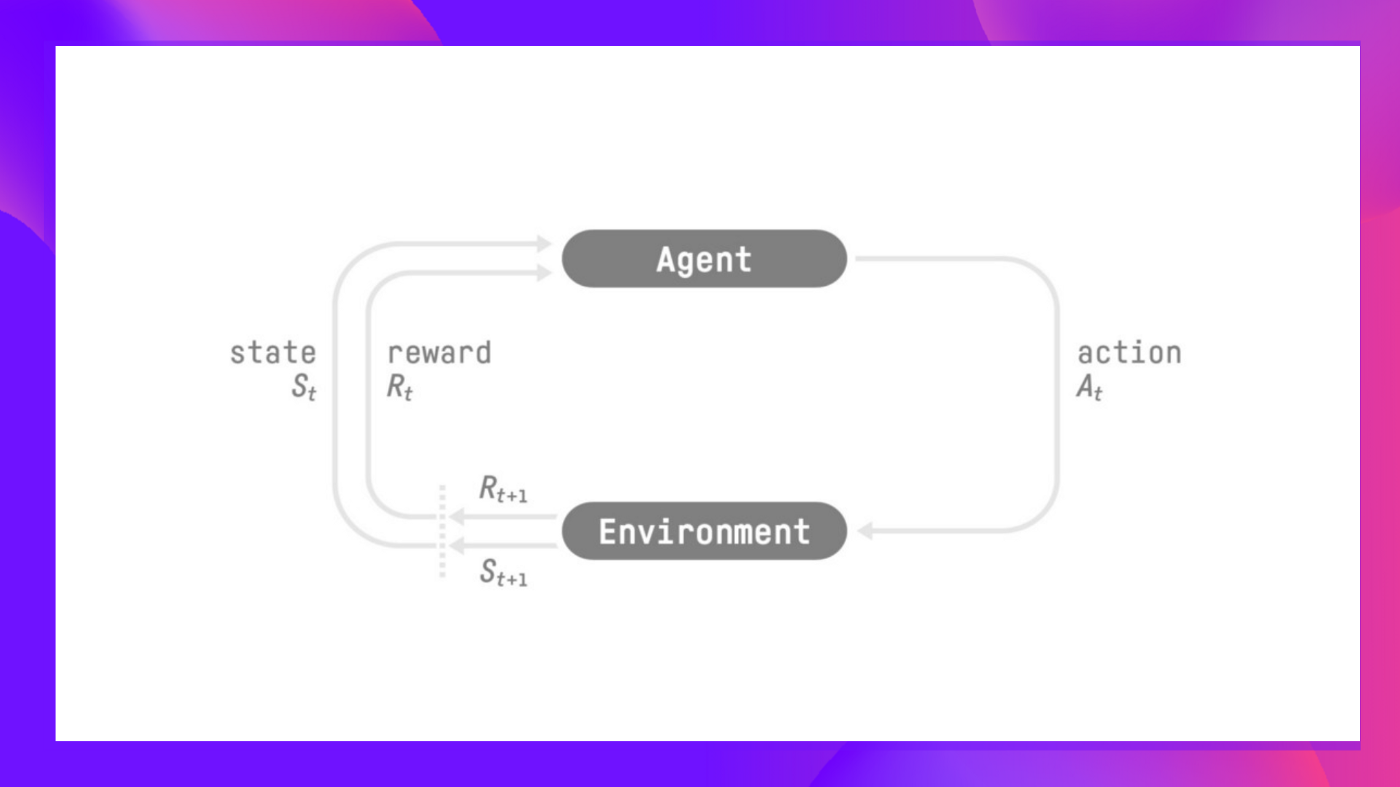
But, to make intelligent decisions, our agent will learn from the environment by interacting with it through trial and error and receiving rewards (positive or negative) as unique feedback.

Its goal is to maximize its expected cumulative reward (because of the reward hypothesis).

The agent's decision-making process is called the policy π: given a state, a policy will output an action or a probability distribution over actions. That is, given an observation of the environment, a policy will provide an action (or multiple probabilities for each action) that the agent should take.

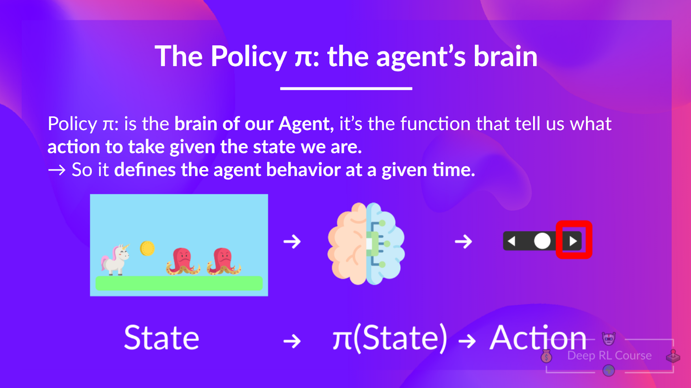
Our goal is to find an optimal policy π*, aka., a policy that leads to the best expected cumulative reward.

And to find this optimal policy (hence solving the RL problem), there are two main types of RL methods:

• Policy-based methods: Train the policy directly to learn which action to take given a state.
• Value-based methods: Train a value function to learn which state is more valuable and use this value function to take the action that leads to it.

And in this chapter, we'll dive deeper into the Value-based methods.

The two types of value-based methods

In value-based methods, we learn a value function that maps a state to the expected value of being at that state.

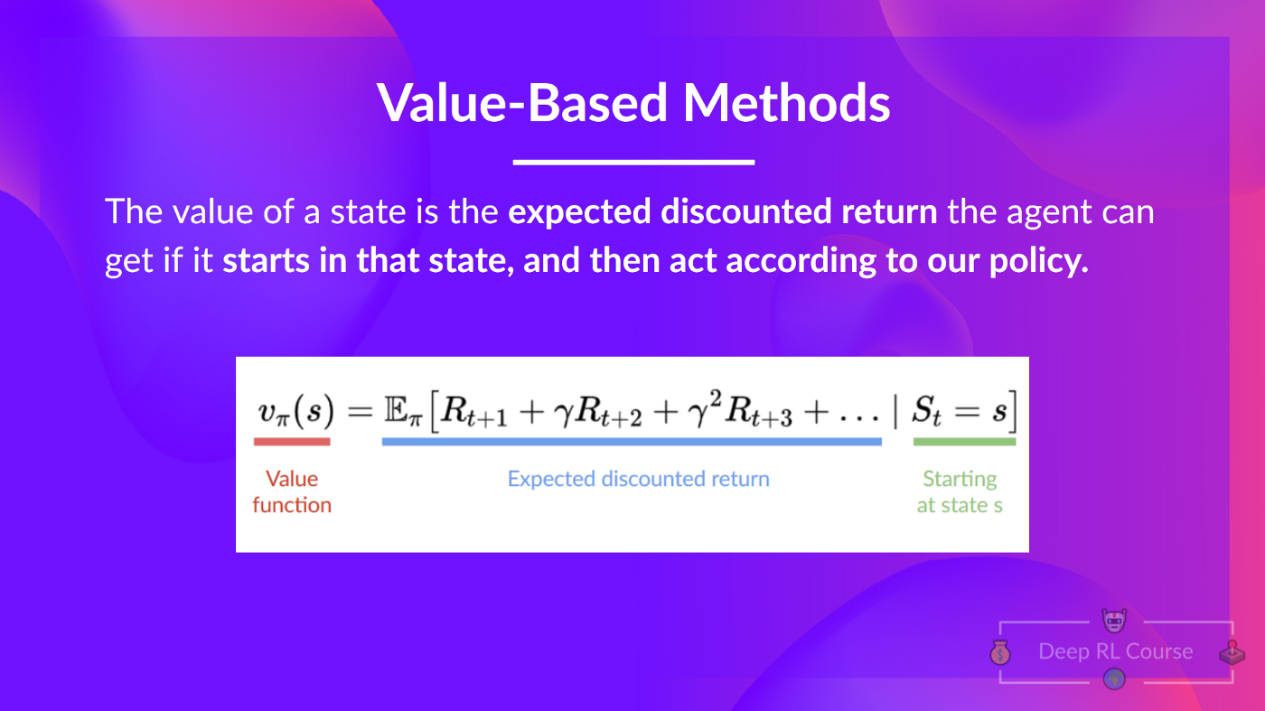
The value of a state is the expected discounted return the agent can get if it starts at that state and then acts according to our policy.

If you forgot what discounting is, you can read this section.

But what does it mean to act according to our policy? After all, we don't have a policy in value-based methods, since we train a value function and not a policy.

Remember that the goal of an RL agent is to have an optimal policy π.

To find it, we learned that there are two different methods:

• Policy-based methods: Directly train the policy to select what action to take given a state (or a probability distribution over actions at that state). In this case, we don't have a value function.

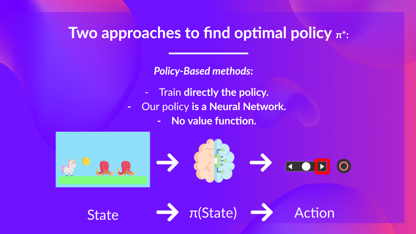
The policy takes a state as input and outputs what action to take at that state (deterministic policy).

And consequently, we don't define by hand the behavior of our policy; it's the training that will define it.

• Value-based methods: Indirectly, by training a value function that outputs the value of a state or a state-action pair. Given this value function, our policy will take action.

But, because we didn't train our policy, we need to specify its behavior. For instance, if we want a policy that, given the value function, will take actions that always lead to the biggest reward, we'll create a Greedy Policy.

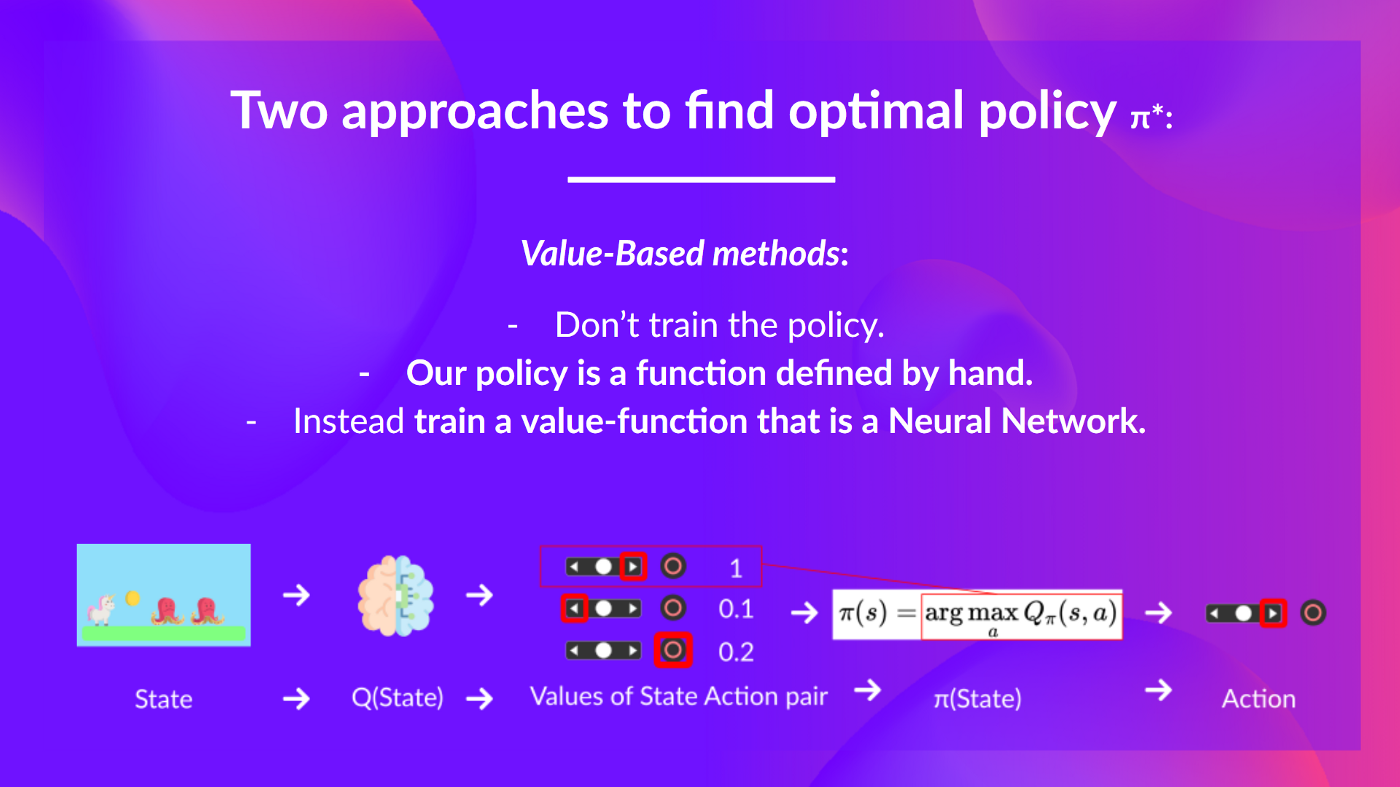
Consequently, whatever method you use to solve your problem, you will have a policy, but in the case of value-based methods you don't train it, your policy is just a simple function that you specify (for instance greedy policy) and this policy uses the values given by the value-function to select its actions.

So the difference is:

• In policy-based, the optimal policy is found by training the policy directly.
• In value-based, finding an optimal value function leads to having an optimal policy.

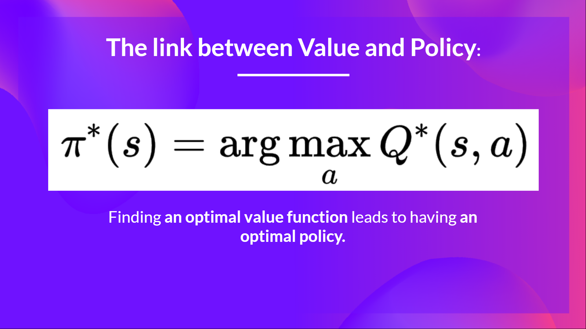
In fact, most of the time, in value-based methods, you'll use an Epsilon-Greedy Policy that handles the exploration/exploitation trade-off; we'll talk about it when we talk about Q-Learning in the second part of this unit.

So, we have two types of value-based functions:

The State-Value function

We write the state value function under a policy π like this:

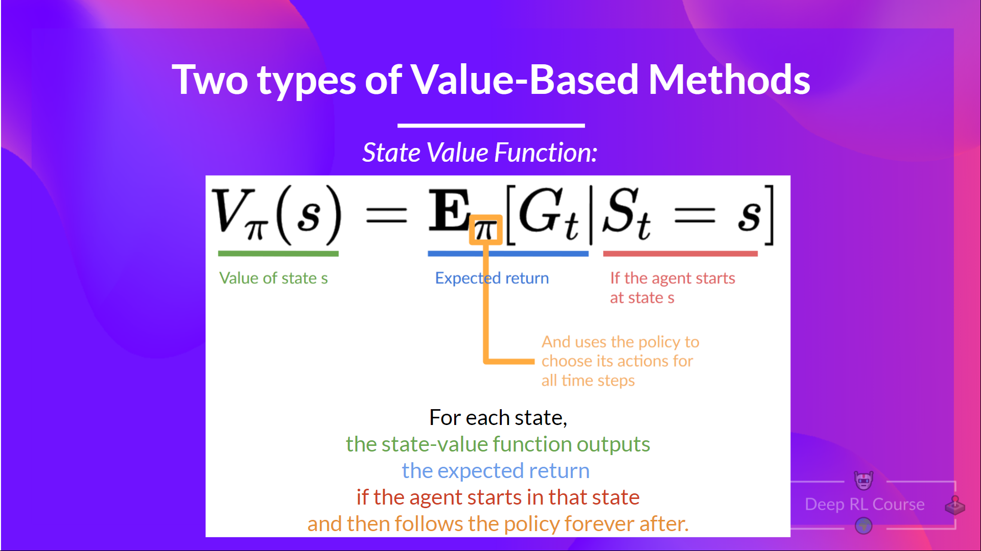
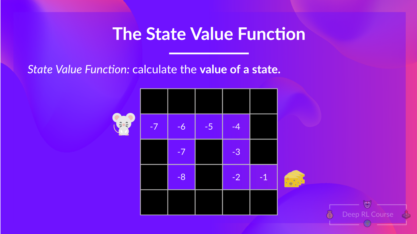
For each state, the state-value function outputs the expected return if the agent starts at that state, and then follow the policy forever after (for all future timesteps if you prefer).

The Action-Value function

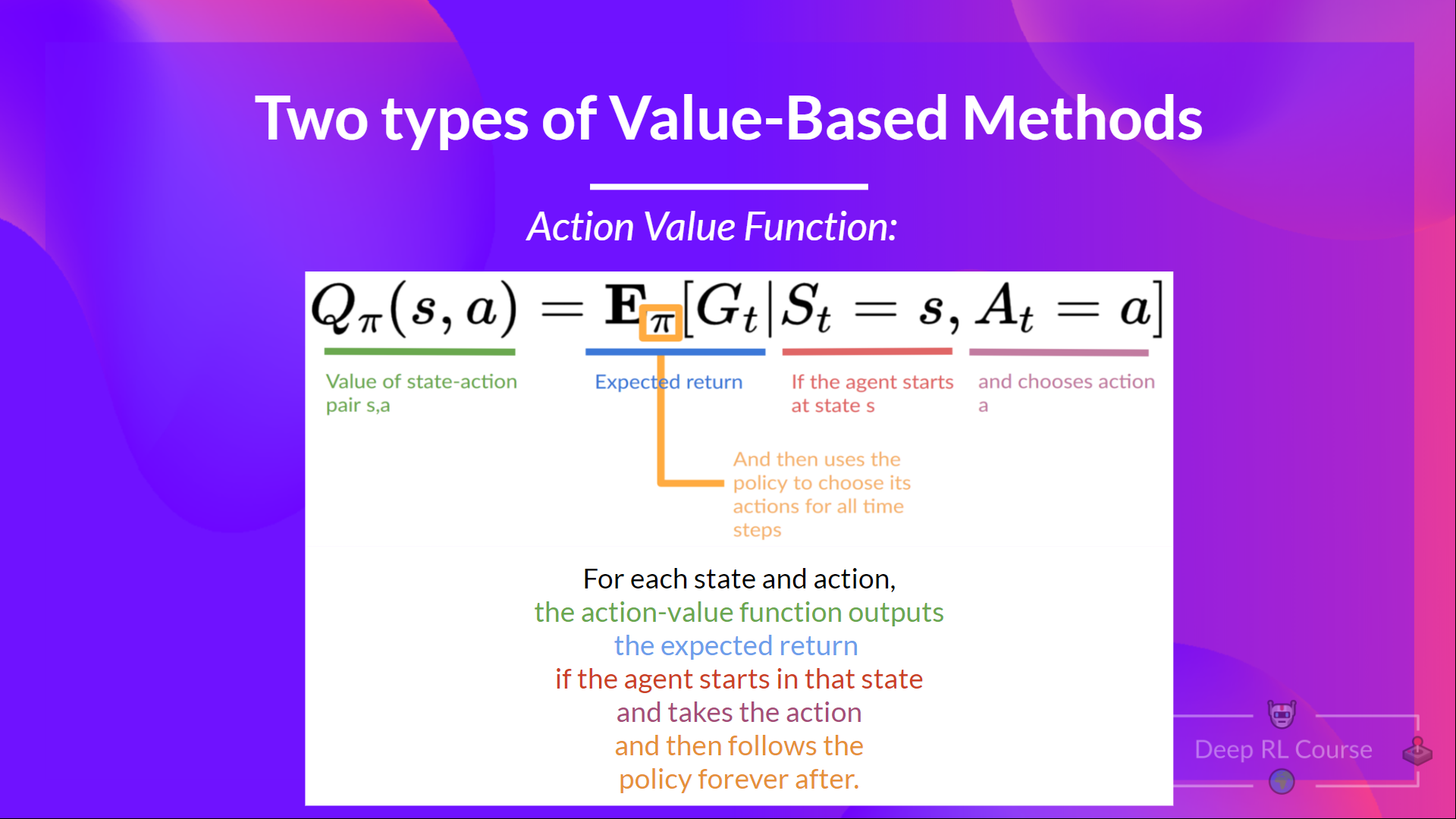
In the Action-value function, for each state and action pair, the action-value function outputs the expected return if the agent starts in that state and takes action, and then follows the policy forever after.

The value of taking action an in state s under a policy π is:

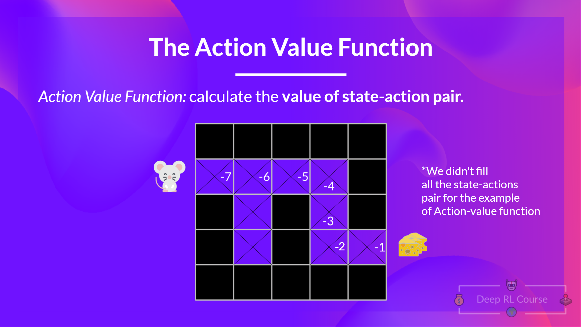
We see that the difference is:

• In state-value function, we calculate the value of a state $S_{t}S\_t$
• In action-value function, we calculate the value of the state-action pair ( $S_t,A_{t}S\_t,\; A\_t$ ) hence the value of taking that action at that state.

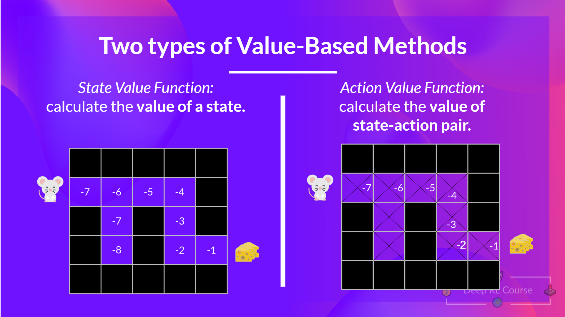
In either case, whatever value function we choose (state-value or action-value function), the value is the expected return.

However, the problem is that it implies that to calculate EACH value of a state or a state-action pair, we need to sum all the rewards an agent can get if it starts at that state.

This can be a tedious process, and that's where the Bellman equation comes to help us.

The Bellman Equation: simplify our value estimation

The Bellman equation simplifies our state value or state-action value calculation.

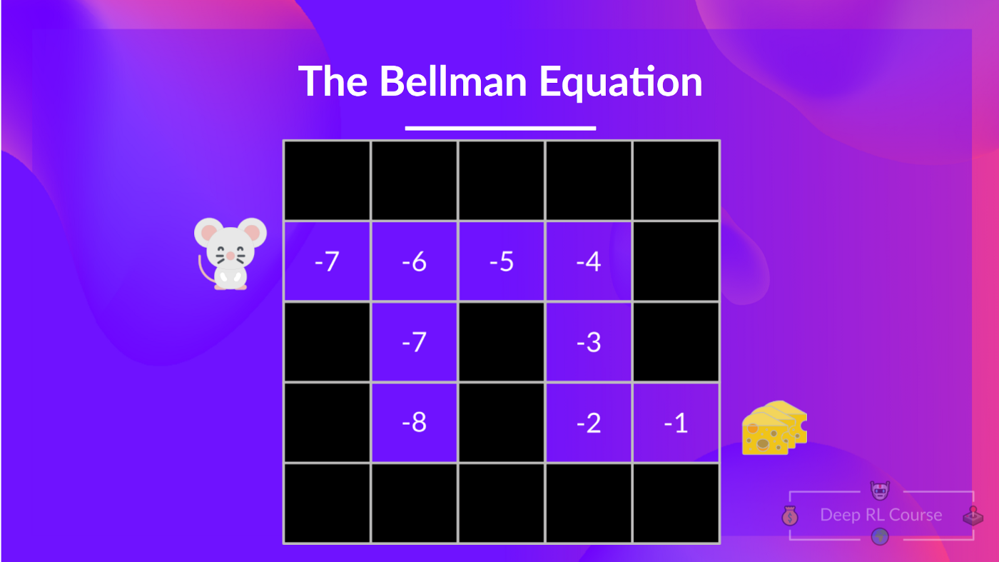
With what we learned from now, we know that if we calculate the $V(S_t)V(S\_t)$ (value of a state), we need to calculate the return starting at that state and then follow the policy forever after. (Our policy that we defined in the following example is a Greedy Policy, and for simplification, we don't discount the reward).

So to calculate $V(S_t)V(S\_t)$, we need to make the sum of the expected rewards. Hence:

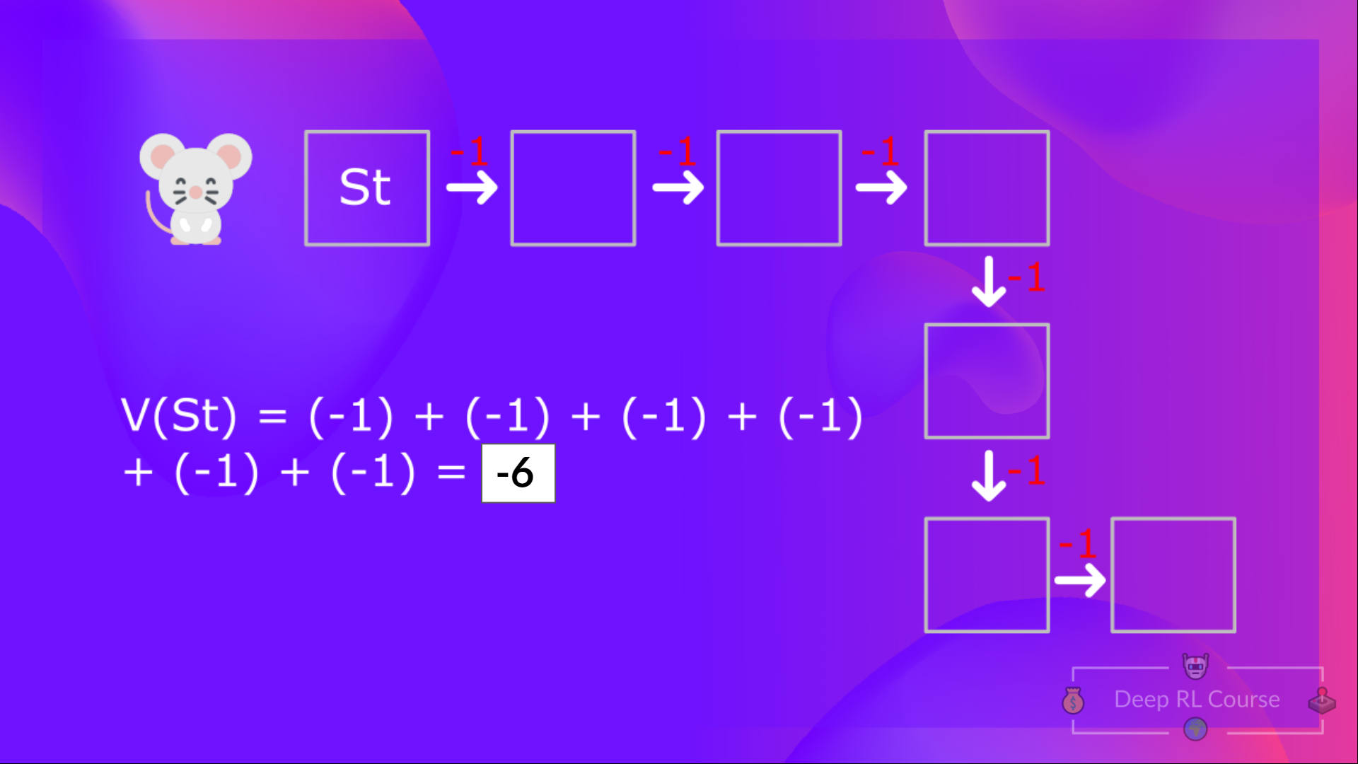
Then, to calculate the $V(S_{t+1})V(S\_\{t+1\})$, we need to calculate the return starting at that state $S_{t+1}S\_\{t+1\}$.

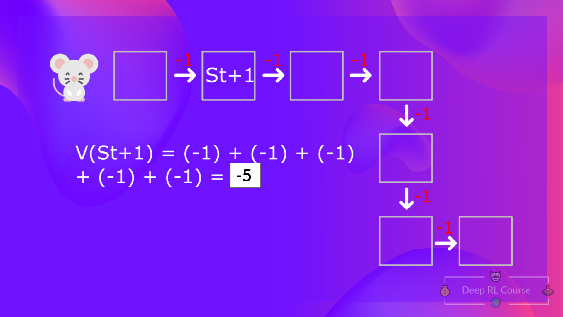
So you see, that's a pretty tedious process if you need to do it for each state value or state-action value.

Instead of calculating the expected return for each state or each state-action pair, we can use the Bellman equation.

The Bellman equation is a recursive equation that works like this: instead of starting for each state from the beginning and calculating the return, we can consider the value of any state as:

The immediate reward $R_{t+1}R\_\{t+1\}$ + the discounted value of the state that follows ( $gamma\ast V(S_{t+1})gamma\; *\; V(S\_\{t+1\})$ ) .

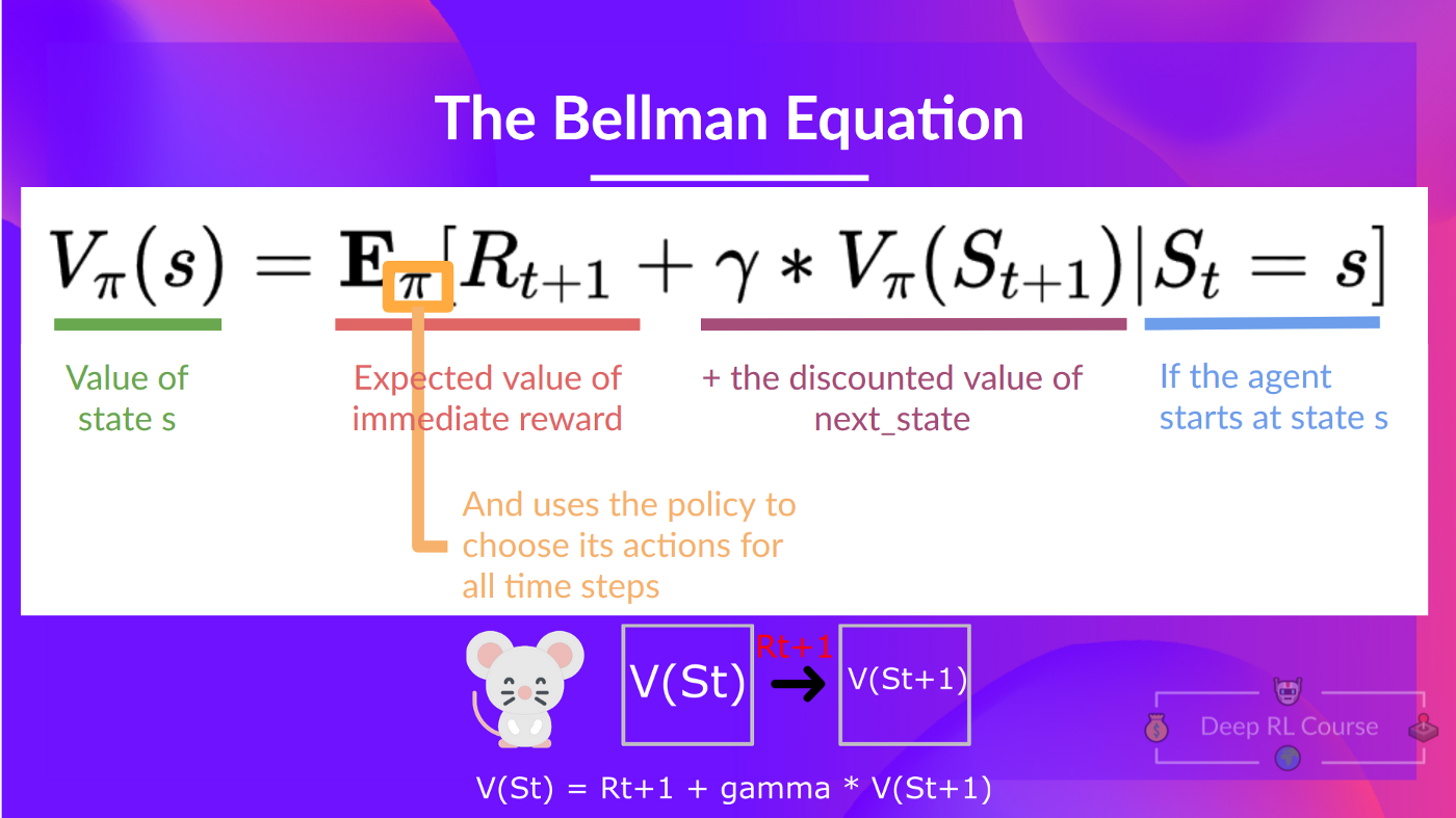
If we go back to our example, the value of State 1= expected cumulative return if we start at that state.

To calculate the value of State 1: the sum of rewards if the agent started in that state 1 and then followed the policy for all the time steps.

Which is equivalent to $V(S_t)V(S\_\{t\})$ = Immediate reward $R_{t+1}R\_\{t+1\}$ + Discounted value of the next state $gamma\ast V(S_{t+1})gamma\; *\; V(S\_\{t+1\})$

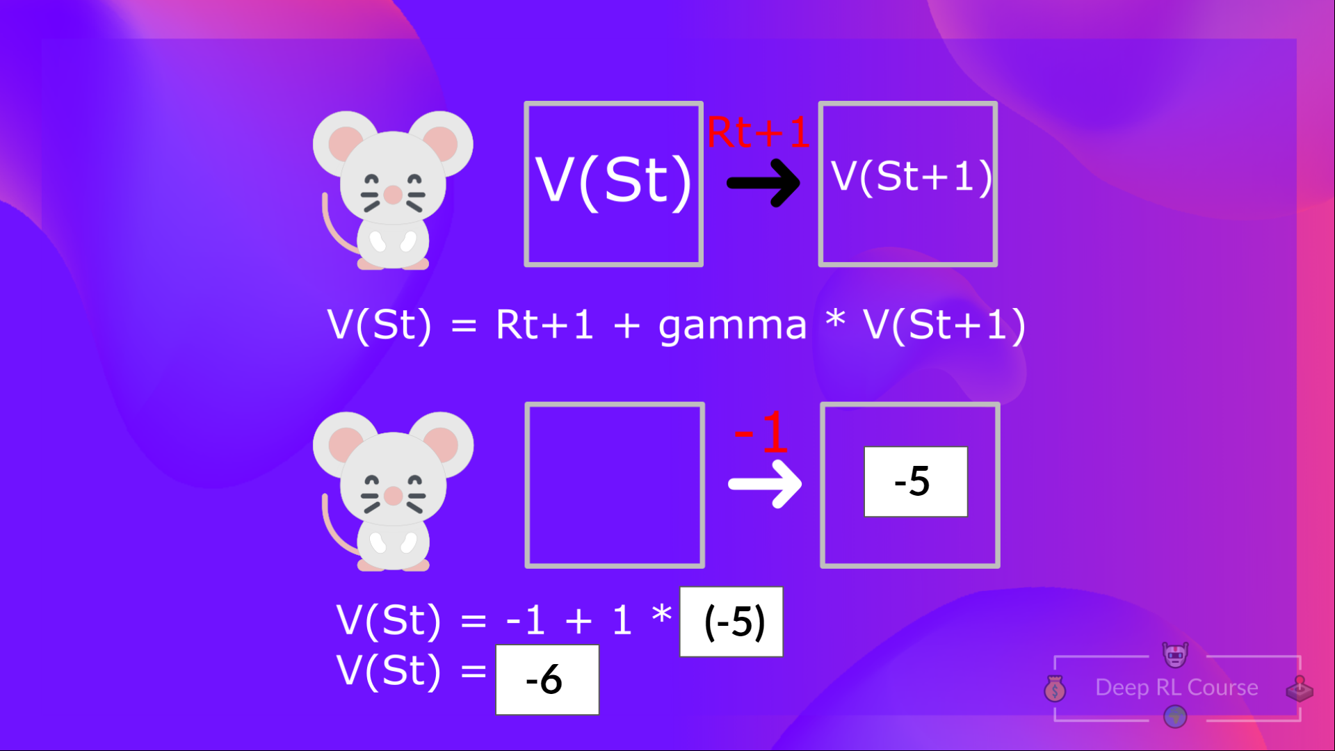
For simplification, here we don't discount, so gamma = 1.

• The value of $V(S_{t+1})V(S\_\{t+1\})$ = Immediate reward $R_{t+2}R\_\{t+2\}$ + Discounted value of the next state ( $gamma\ast V(S_{t+2})gamma\; *\; V(S\_\{t+2\})$ ).
• And so on.

To recap, the idea of the Bellman equation is that instead of calculating each value as the sum of the expected return, which is a long process. This is equivalent to the sum of immediate reward + the discounted value of the state that follows.

Monte Carlo vs Temporal Difference Learning

The last thing we need to talk about before diving into Q-Learning is the two ways of learning.

Remember that an RL agent learns by interacting with its environment. The idea is that using the experience taken, given the reward it gets, will update its value or policy.

Monte Carlo and Temporal Difference Learning are two different strategies on how to train our value function or our policy function. Both of them use experience to solve the RL problem.

On one hand, Monte Carlo uses an entire episode of experience before learning. On the other hand, Temporal Difference uses only a step ( $S_t,A_t,R_{t+1},S_{t+1}S\_t,\; A\_t,\; R\_\{t+1\},\; S\_\{t+1\}$ ) to learn.

We'll explain both of them using a value-based method example.

Monte Carlo: learning at the end of the episode

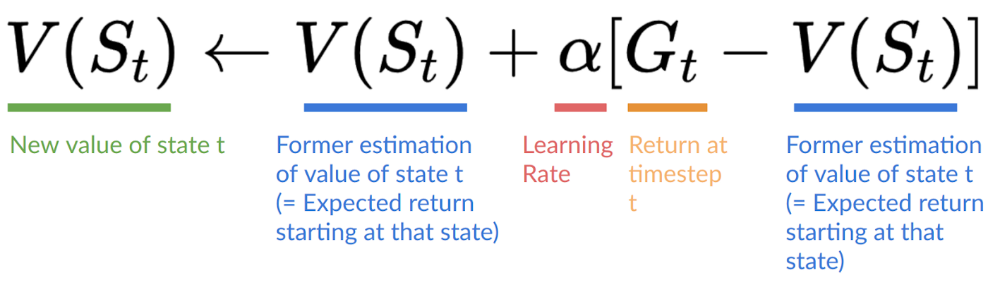
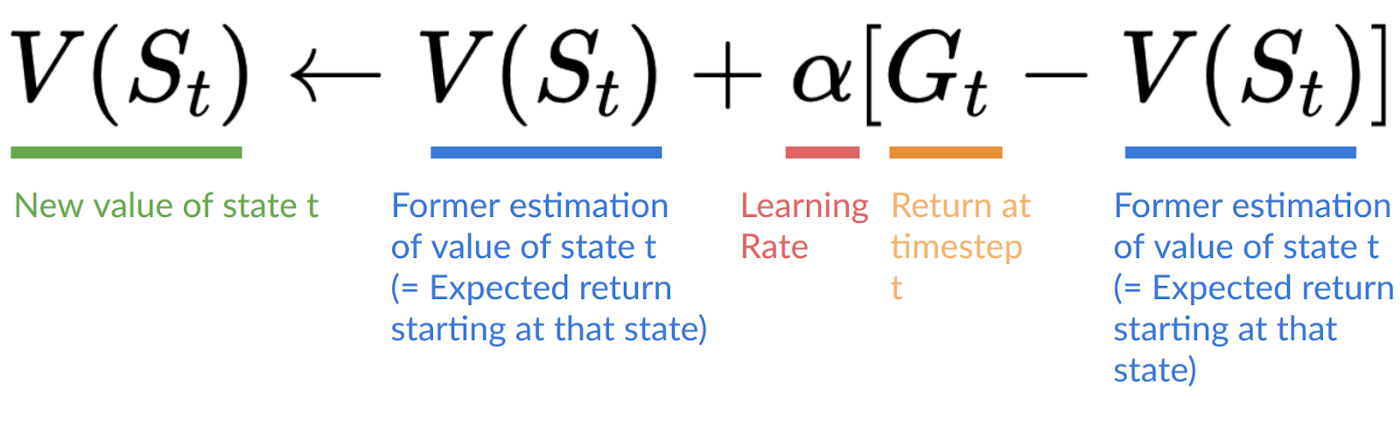
Monte Carlo waits until the end of the episode, calculates $G_{t}G\_t$ (return) and uses it as a target for updating $V(S_t)V(S\_t)$.

So it requires a complete entire episode of interaction before updating our value function.

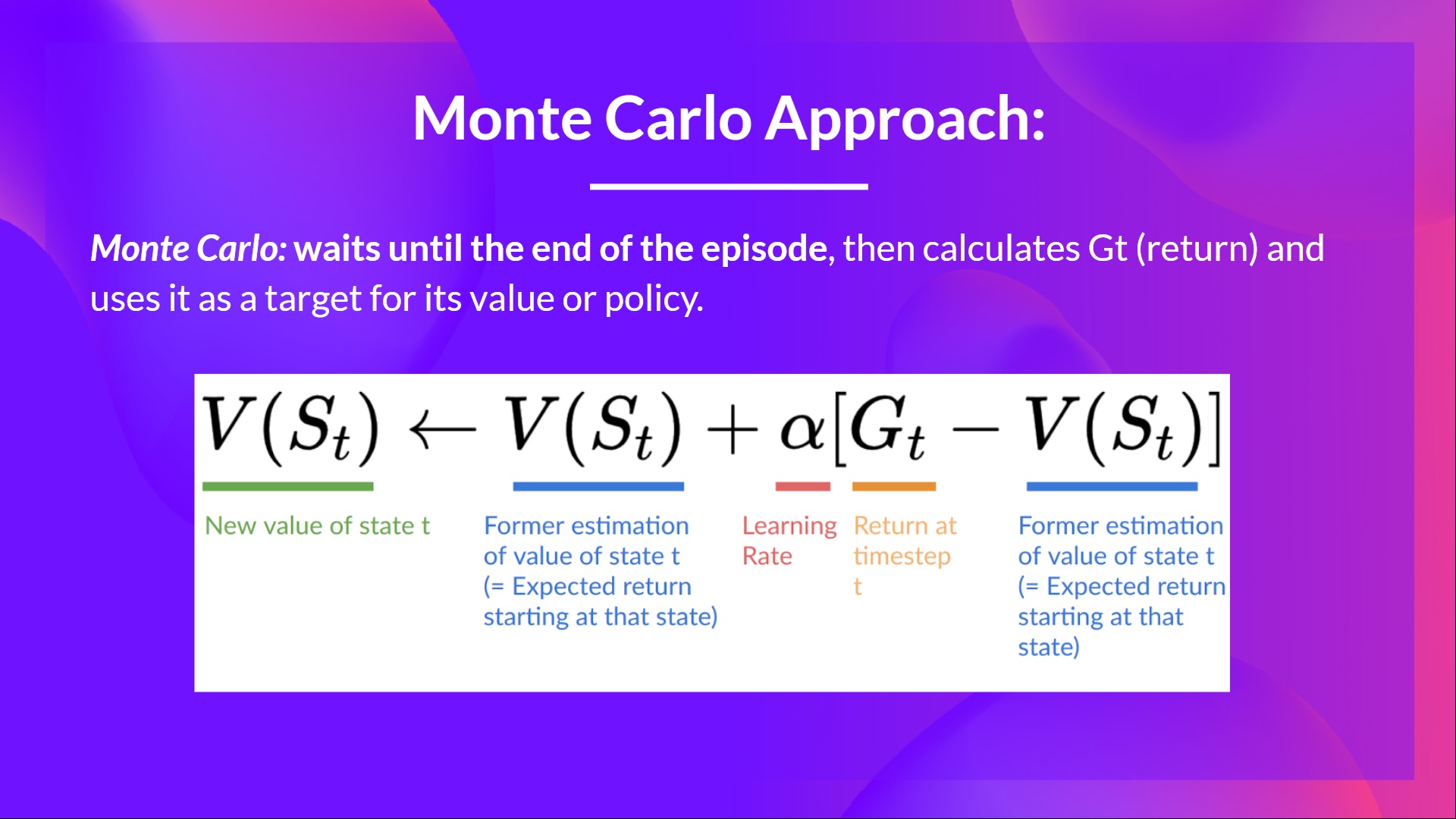
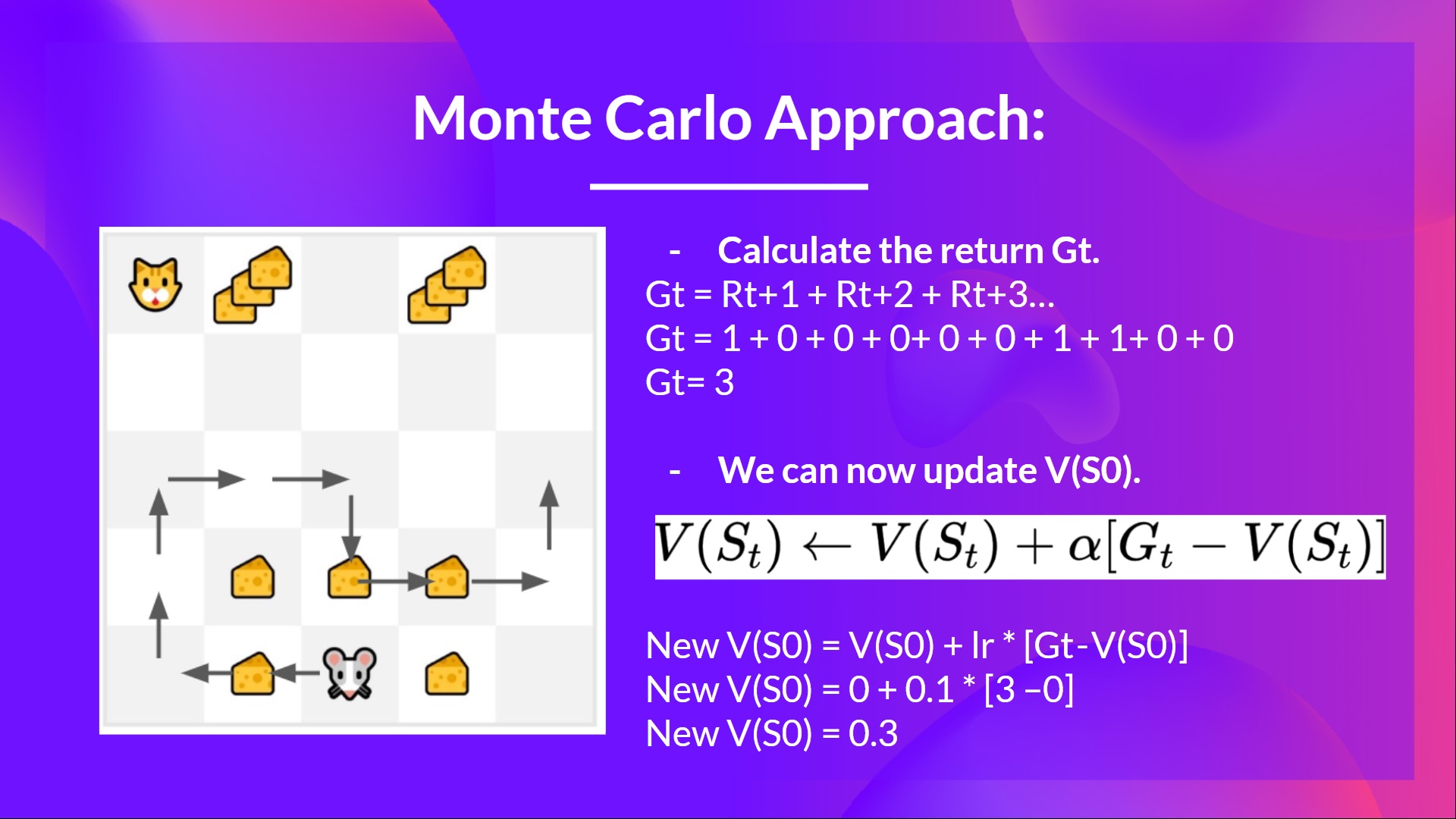
If we take an example:

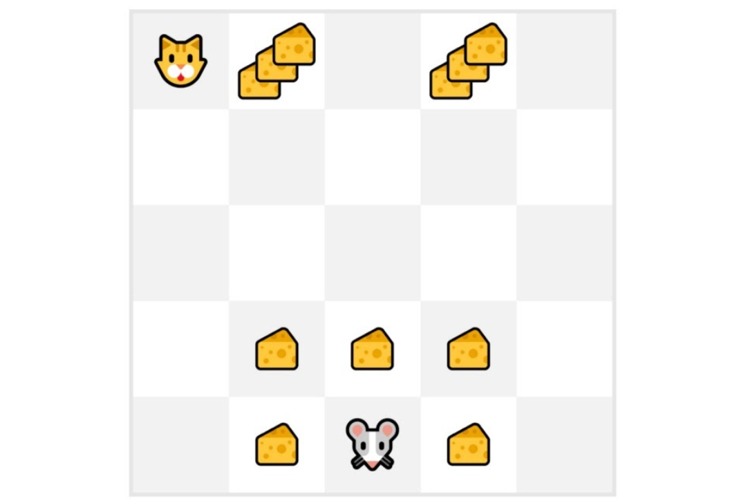
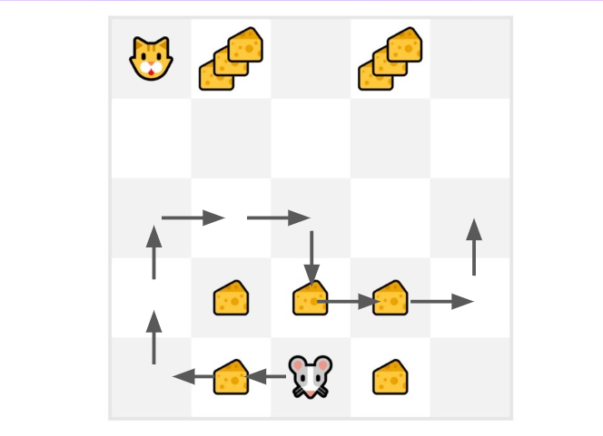
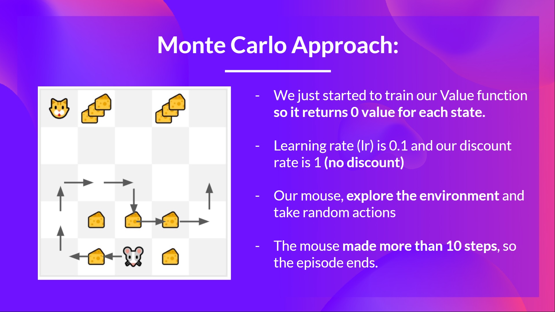
• We always start the episode at the same starting point.

• The agent takes actions using the policy. For instance, using an Epsilon Greedy Strategy, a policy that alternates between exploration (random actions) and exploitation.

• We get the reward and the next state.

• We terminate the episode if the cat eats the mouse or if the mouse moves > 10 steps.

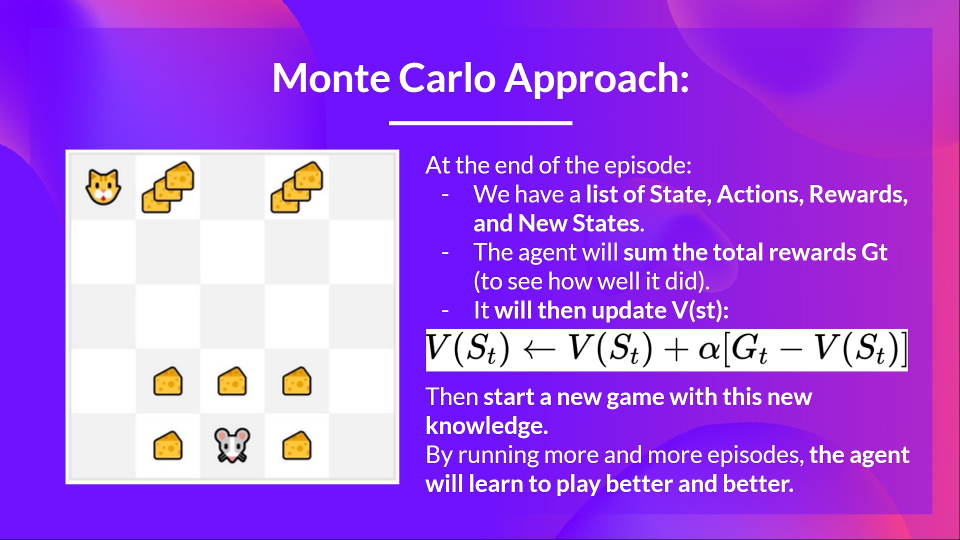
• At the end of the episode, we have a list of State, Actions, Rewards, and Next States

• The agent will sum the total rewards $G_{t}G\_t$ (to see how well it did).

• It will then update $V(s_t)V(s\_t)$ based on the formula

• Then start a new game with this new knowledge

By running more and more episodes, the agent will learn to play better and better.

For instance, if we train a state-value function using Monte Carlo:

• We just started to train our Value function, so it returns 0 value for each state
• Our learning rate (lr) is 0.1 and our discount rate is 1 (= no discount)
• Our mouse explores the environment and takes random actions

• The mouse made more than 10 steps, so the episode ends .

• We have a list of state, action, rewards, next_state, we need to calculate the return $GtG\{t\}$
• $G_t=R_{t+1}+R_{t+2}+R_{t+3}\mathrm{.}\mathrm{.}\mathrm{.}G\_t\; =\; R\_\{t+1\}\; +\; R\_\{t+2\}\; +\; R\_\{t+3\}\; ...$
• $G_t=R_{t+1}+R_{t+2}+R_{t+3}\dots G\_t\; =\; R\_\{t+1\}\; +\; R\_\{t+2\}\; +\; R\_\{t+3\}\dots$ (for simplicity we don’t discount the rewards).
• $G_t=1+0+0+0+0+0+1+1+0+0G\_t\; =\; 1\; +\; 0\; +\; 0\; +\; 0+\; 0\; +\; 0\; +\; 1\; +\; 1\; +\; 0\; +\; 0$
• $G_t=3G\_t=\; 3$
• We can now update $V(S_0)V(S\_0)$:

• New $V(S_0)=V(S_0)+lr\ast [G_t\text{—}V(S_0)]V(S\_0)\; =\; V(S\_0)\; +\; lr\; *\; [G\_t\; —\; V(S\_0)]$
• New $V(S_0)=0+0.1\ast [3\text{–}0]V(S\_0)\; =\; 0\; +\; 0.1\; *\; [3\; –\; 0]$
• New $V(S_0)=0.3V(S\_0)\; =\; 0.3$

Temporal Difference Learning: learning at each step

• Temporal difference, on the other hand, waits for only one interaction (one step) $S_{t+1}S\_\{t+1\}$
• to form a TD target and update $V(S_t)V(S\_t)$ using $R_{t+1}R\_\{t+1\}$ and $gamma\ast V(S_{t+1})gamma\; *\; V(S\_\{t+1\})$.

The idea with TD is to update the $V(S_t)V(S\_t)$ at each step.

But because we didn't play during an entire episode, we don't have $G_{t}G\_t$ (expected return). Instead, we estimate $G_{t}G\_t$ by adding $R_{t+1}R\_\{t+1\}$ and the discounted value of the next state.

This is called bootstrapping. It's called this because TD bases its update part on an existing estimate $V(S_{t+1})V(S\_\{t+1\})$ and not a complete sample $G_{t}G\_t$.

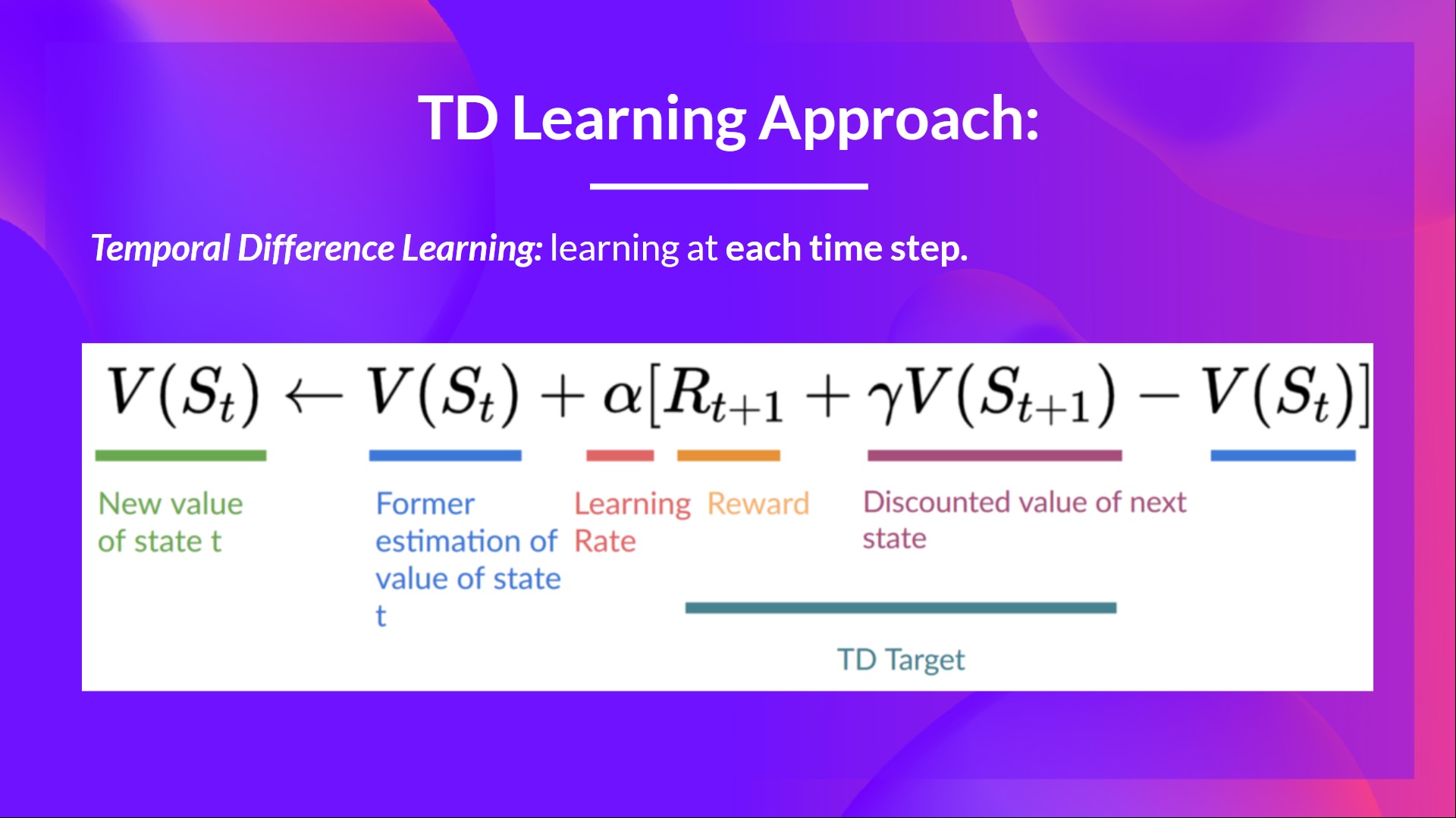
This method is called TD(0) or one-step TD (update the value function after any individual step).

If we take the same example,

• We just started to train our Value function, so it returns 0 value for each state.
• Our learning rate (lr) is 0.1, and our discount rate is 1 (no discount).
• Our mouse explore the environment and take a random action: going to the left
• It gets a reward $R_{t+1}=1R\_\{t+1\}\; =\; 1$ since it eats a piece of cheese

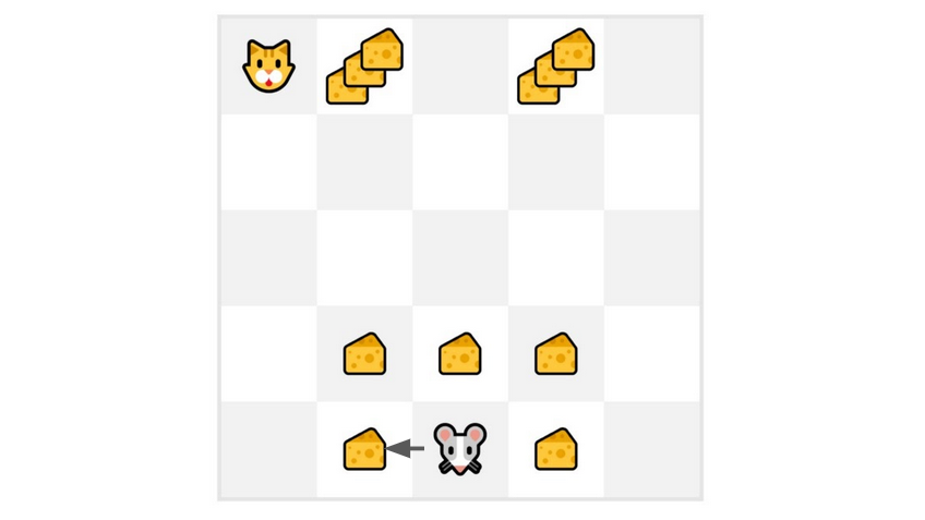
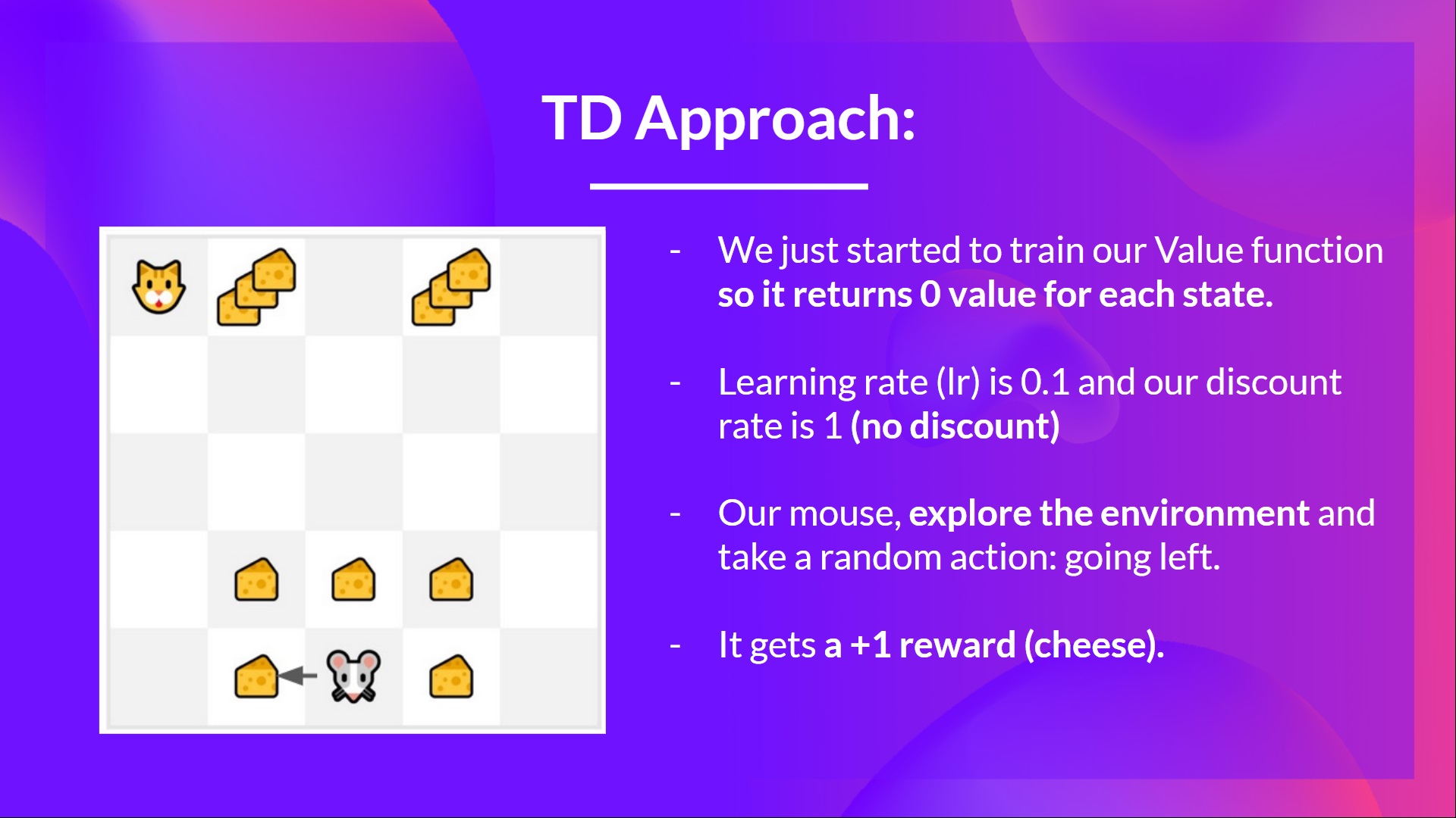
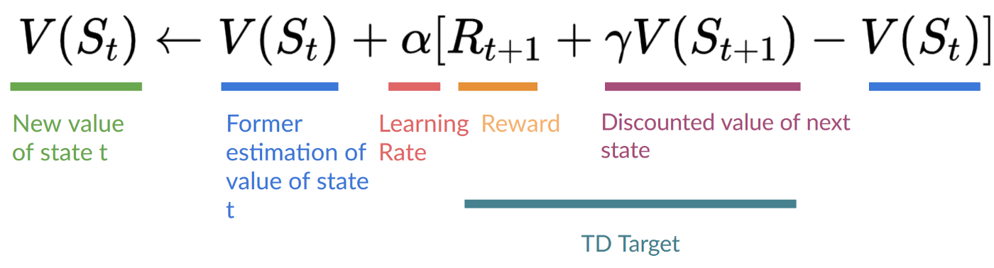
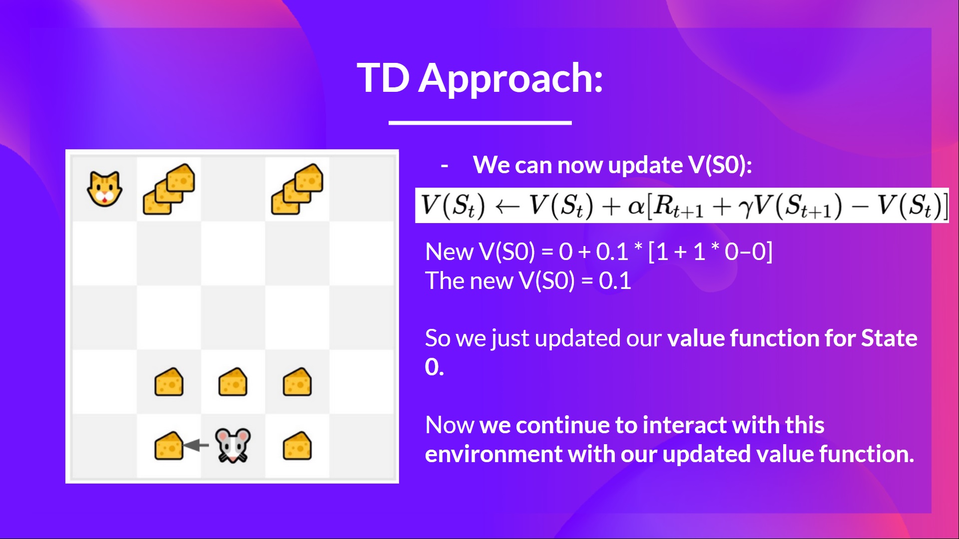
We can now update $V(S_0)V(S\_0)$:

New $V(S_0)=V(S_0)+lr\ast [R_1+gamma\ast V(S_1)-V(S_0)]V(S\_0)\; =\; V(S\_0)\; +\; lr\; *\; [R\_1\; +\; gamma\; *\; V(S\_1)\; -\; V(S\_0)]$

New $V(S_0)=0+0.1\ast [1+1\ast 0\text{–}0]V(S\_0)\; =\; 0\; +\; 0.1\; *\; [1\; +\; 1\; *\; 0–0]$

New $V(S_0)=0.1V(S\_0)\; =\; 0.1$

So we just updated our value function for State 0.

Now we continue to interact with this environment with our updated value function.

If we summarize:

• With Monte Carlo, we update the value function from a complete episode, and so we use the actual accurate discounted return of this episode.
• With TD learning, we update the value function from a step, so we replace $G_{t}G\_t$ that we don't have with an estimated return called TD target.

So now, before diving on Q-Learning, let's summarise what we just learned:

We have two types of value-based functions:

• State-Value function: outputs the expected return if the agent starts at a given state and acts accordingly to the policy forever after.
• Action-Value function: outputs the expected return if the agent starts in a given state, takes a given action at that state and then acts accordingly to the policy forever after.
• In value-based methods, we define the policy by hand because we don't train it, we train a value function. The idea is that if we have an optimal value function, we will have an optimal policy.

There are two types of methods to learn a policy for a value function:

• With the Monte Carlo method, we update the value function from a complete episode, and so we use the actual accurate discounted return of this episode.
• With the TD Learning method, we update the value function from a step, so we replace Gt that we don't have with an estimated return called TD target.

---

So that’s all for today. Congrats on finishing this first part of the chapter! There was a lot of information.

That’s normal if you still feel confused with all these elements. This was the same for me and for all people who studied RL.

Take time to really grasp the material before continuing.

And since the best way to learn and avoid the illusion of competence is to test yourself. We wrote a quiz to help you find where you need to reinforce your study. Check your knowledge here 👉 https://github.com/huggingface/deep-rl-class/blob/main/unit2/quiz1.md

In the second part , we’ll study our first RL algorithm: Q-Learning, and implement our first RL Agent in two environments:

1. Frozen-Lake-v1 (non-slippery version): where our agent will need to go from the starting state (S) to the goal state (G) by walking only on frozen tiles (F) and avoiding holes (H).
2. An autonomous taxi will need to learn to navigate a city to transport its passengers from point A to point B.

And don't forget to share with your friends who want to learn 🤗 !

Finally, we want to improve and update the course iteratively with your feedback. If you have some, please fill this form 👉 https://forms.gle/3HgA7bEHwAmmLfwh9

Keep learning, stay awesome,