Back to Articles

This article is also available in Chinese 简体中文.

Note: Edited on July 2023 with up-to-date references and examples.

Introduction

In recent years, there has been an increasing interest in open-ended language generation thanks to the rise of large transformer-based language models trained on millions of webpages, including OpenAI's ChatGPT and Meta's LLaMA. The results on conditioned open-ended language generation are impressive, having shown to generalize to new tasks, handle code, or take non-text data as input. Besides the improved transformer architecture and massive unsupervised training data, better decoding methods have also played an important role.

This blog post gives a brief overview of different decoding strategies and more importantly shows how you can implement them with very little effort using the popular transformers library!

All of the following functionalities can be used for auto-regressive language generation (here a refresher). In short, auto-regressive language generation is based on the assumption that the probability distribution of a word sequence can be decomposed into the product of conditional next word distributions:

$$P(w_{1:T}\mathrm{\mid }{W}_0)=\prod _{t=1}^{T}P(w_t\mathrm{\mid }{w}_{1:t-1},W_0)\text{ ,with }{w}_{1:0}=\mathrm{\varnothing },P(w\_\{1:T\}\; |\; W\_0\; )\; =\; \backslash prod\_\{t=1\}^T\; P(w\_\{t\}\; |\; w\_\{1:\; t-1\},\; W\_0)\; \backslash text\{\; ,with\; \}\; w\_\{1:\; 0\}\; =\; \backslash emptyset,$$

and $W_{0}W\_0$ being the initial context word sequence. The length $TT$ of the word sequence is usually determined on-the-fly and corresponds to the timestep $t=Tt=T$ the EOS token is generated from $P(w_t\mathrm{\mid }{w}_{1:t-1},W_0)P(w\_\{t\}\; |\; w\_\{1:\; t-1\},\; W\_\{0\})$.

We will give a tour of the currently most prominent decoding methods, mainly Greedy search, Beam search, and Sampling.

Let's quickly install transformers and load the model. We will use GPT2 in PyTorch for demonstration, but the API is 1-to-1 the same for TensorFlow and JAX.

!pip install -q transformers

from transformers import AutoModelForCausalLM, AutoTokenizer
import torch

torch_device = "cuda" if torch.cuda.is_available() else "cpu"

tokenizer = AutoTokenizer.from_pretrained("gpt2")

# add the EOS token as PAD token to avoid warnings
model = AutoModelForCausalLM.from_pretrained("gpt2", pad_token_id=tokenizer.eos_token_id).to(torch_device)

Greedy Search

Greedy search is the simplest decoding method. It selects the word with the highest probability as its next word: $w_t=argma{x}_{w}P(w\mathrm{\mid }{w}_{1:t-1})w\_t\; =\; argmax\_\{w\}P(w\; |\; w\_\{1:t-1\})$ at each timestep $tt$. The following sketch shows greedy search.

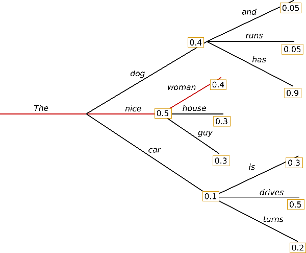
Starting from the word $\text{"The"},\backslash text\{"The"\},$ the algorithm greedily chooses the next word of highest probability $\text{"nice"}\backslash text\{"nice"\}$ and so on, so that the final generated word sequence is $(\text{"The"},\text{"nice"},\text{"woman"})(\backslash text\{"The"\},\; \backslash text\{"nice"\},\; \backslash text\{"woman"\})$ having an overall probability of $0.5\times 0.4=0.20.5\; \backslash times\; 0.4\; =\; 0.2$ .

In the following we will generate word sequences using GPT2 on the context $(\text{"I"},\text{"enjoy"},\text{"walking"},\text{"with"},\text{"my"},\text{"cute"},\text{"dog"})(\backslash text\{"I"\},\; \backslash text\{"enjoy"\},\; \backslash text\{"walking"\},\; \backslash text\{"with"\},\; \backslash text\{"my"\},\; \backslash text\{"cute"\},\; \backslash text\{"dog"\})$. Let's see how greedy search can be used in transformers:

# encode context the generation is conditioned on
model_inputs = tokenizer('I enjoy walking with my cute dog', return_tensors='pt').to(torch_device)

# generate 40 new tokens
greedy_output = model.generate(**model_inputs, max_new_tokens=40)

print("Output:\n" + 100 * '-')
print(tokenizer.decode(greedy_output[0], skip_special_tokens=True))

Output:
----------------------------------------------------------------------------------------------------
I enjoy walking with my cute dog, but I'm not sure if I'll ever be able to walk with my dog. I'm not sure if I'll ever be able to walk with my dog.

I'm not sure

Alright! We have generated our first short text with GPT2 😊. The generated words following the context are reasonable, but the model quickly starts repeating itself! This is a very common problem in language generation in general and seems to be even more so in greedy and beam search - check out Vijayakumar et al., 2016 and Shao et al., 2017.

The major drawback of greedy search though is that it misses high probability words hidden behind a low probability word as can be seen in our sketch above:

The word $\text{"has"}\backslash text\{"has"\}$ with its high conditional probability of $0.90.9$ is hidden behind the word $\text{"dog"}\backslash text\{"dog"\}$, which has only the second-highest conditional probability, so that greedy search misses the word sequence $\text{"The"},\text{"dog"},\text{"has"}\backslash text\{"The"\},\; \backslash text\{"dog"\},\; \backslash text\{"has"\}$ .

Thankfully, we have beam search to alleviate this problem!

Beam search

Beam search reduces the risk of missing hidden high probability word sequences by keeping the most likely num_beams of hypotheses at each time step and eventually choosing the hypothesis that has the overall highest probability. Let's illustrate with num_beams=2:

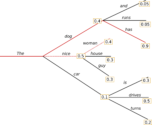
At time step 1, besides the most likely hypothesis $(\text{"The"},\text{"nice"})(\backslash text\{"The"\},\; \backslash text\{"nice"\})$, beam search also keeps track of the second most likely one $(\text{"The"},\text{"dog"})(\backslash text\{"The"\},\; \backslash text\{"dog"\})$. At time step 2, beam search finds that the word sequence $(\text{"The"},\text{"dog"},\text{"has"})(\backslash text\{"The"\},\; \backslash text\{"dog"\},\; \backslash text\{"has"\})$, has with $0.360.36$ a higher probability than $(\text{"The"},\text{"nice"},\text{"woman"})(\backslash text\{"The"\},\; \backslash text\{"nice"\},\; \backslash text\{"woman"\})$, which has $0.20.2$ . Great, it has found the most likely word sequence in our toy example!

Beam search will always find an output sequence with higher probability than greedy search, but is not guaranteed to find the most likely output.

Let's see how beam search can be used in transformers. We set num_beams > 1 and early_stopping=True so that generation is finished when all beam hypotheses reached the EOS token.

# activate beam search and early_stopping
beam_output = model.generate(
    **model_inputs,
    max_new_tokens=40,
    num_beams=5,
    early_stopping=True
)

print("Output:\n" + 100 * '-')
print(tokenizer.decode(beam_output[0], skip_special_tokens=True))

Output:
----------------------------------------------------------------------------------------------------
I enjoy walking with my cute dog, but I'm not sure if I'll ever be able to walk with him again.

I'm not sure if I'll ever be able to walk with him again. I'm not sure

While the result is arguably more fluent, the output still includes repetitions of the same word sequences. One of the available remedies is to introduce n-grams (a.k.a word sequences of n words) penalties as introduced by Paulus et al. (2017) and Klein et al. (2017). The most common n-grams penalty makes sure that no n-gram appears twice by manually setting the probability of next words that could create an already seen n-gram to 0.

Let's try it out by setting no_repeat_ngram_size=2 so that no 2-gram appears twice:

# set no_repeat_ngram_size to 2
beam_output = model.generate(
    **model_inputs,
    max_new_tokens=40,
    num_beams=5,
    no_repeat_ngram_size=2,
    early_stopping=True
)

print("Output:\n" + 100 * '-')
print(tokenizer.decode(beam_output[0], skip_special_tokens=True))

Output:
----------------------------------------------------------------------------------------------------
I enjoy walking with my cute dog, but I'm not sure if I'll ever be able to walk with him again.

I've been thinking about this for a while now, and I think it's time for me to

Nice, that looks much better! We can see that the repetition does not appear anymore. Nevertheless, n-gram penalties have to be used with care. An article generated about the city New York should not use a 2-gram penalty or otherwise, the name of the city would only appear once in the whole text!

Another important feature about beam search is that we can compare the top beams after generation and choose the generated beam that fits our purpose best.

In transformers, we simply set the parameter num_return_sequences to the number of highest scoring beams that should be returned. Make sure though that num_return_sequences <= num_beams!

# set return_num_sequences > 1
beam_outputs = model.generate(
    **model_inputs,
    max_new_tokens=40,
    num_beams=5,
    no_repeat_ngram_size=2,
    num_return_sequences=5,
    early_stopping=True
)

# now we have 3 output sequences
print("Output:\n" + 100 * '-')
for i, beam_output in enumerate(beam_outputs):
  print("{}: {}".format(i, tokenizer.decode(beam_output, skip_special_tokens=True)))

Output:
----------------------------------------------------------------------------------------------------
0: I enjoy walking with my cute dog, but I'm not sure if I'll ever be able to walk with him again.

I've been thinking about this for a while now, and I think it's time for me to
1: I enjoy walking with my cute dog, but I'm not sure if I'll ever be able to walk with her again.

I've been thinking about this for a while now, and I think it's time for me to
2: I enjoy walking with my cute dog, but I'm not sure if I'll ever be able to walk with him again.

I've been thinking about this for a while now, and I think it's a good idea to
3: I enjoy walking with my cute dog, but I'm not sure if I'll ever be able to walk with him again.

I've been thinking about this for a while now, and I think it's time to take a
4: I enjoy walking with my cute dog, but I'm not sure if I'll ever be able to walk with him again.

I've been thinking about this for a while now, and I think it's a good idea.

As can be seen, the five beam hypotheses are only marginally different to each other - which should not be too surprising when using only 5 beams.

In open-ended generation, a couple of reasons have been brought forward why beam search might not be the best possible option:

• Beam search can work very well in tasks where the length of the desired generation is more or less predictable as in machine translation or summarization - see Murray et al. (2018) and Yang et al. (2018). But this is not the case for open-ended generation where the desired output length can vary greatly, e.g. dialog and story generation.

• We have seen that beam search heavily suffers from repetitive generation. This is especially hard to control with n-gram- or other penalties in story generation since finding a good trade-off between inhibiting repetition and repeating cycles of identical n-grams requires a lot of finetuning.

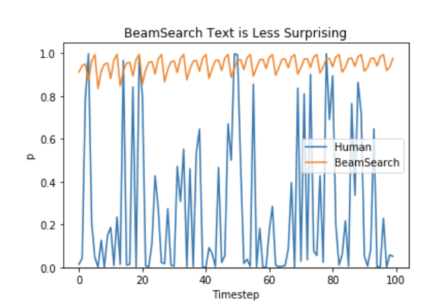
• As argued in Ari Holtzman et al. (2019), high quality human language does not follow a distribution of high probability next words. In other words, as humans, we want generated text to surprise us and not to be boring/predictable. The authors show this nicely by plotting the probability, a model would give to human text vs. what beam search does.

So let's stop being boring and introduce some randomness 🤪.

Sampling

In its most basic form, sampling means randomly picking the next word $w_{t}w\_t$ according to its conditional probability distribution:

$$w_t\sim P(w\mathrm{\mid }{w}_{1:t-1})w\_t\; \backslash sim\; P(w|w\_\{1:t-1\})$$

Taking the example from above, the following graphic visualizes language generation when sampling.

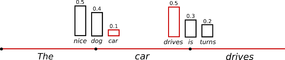
It becomes obvious that language generation using sampling is not deterministic anymore. The word $(\text{"car"})(\backslash text\{"car"\})$ is sampled from the conditioned probability distribution $P(w\mathrm{\mid }\text{"The"})P(w\; |\; \backslash text\{"The"\})$, followed by sampling $(\text{"drives"})(\backslash text\{"drives"\})$ from $P(w\mathrm{\mid }\text{"The"},\text{"car"})P(w\; |\; \backslash text\{"The"\},\; \backslash text\{"car"\})$ .

In transformers, we set do_sample=True and deactivate Top-K sampling (more on this later) via top_k=0. In the following, we will fix the random seed for illustration purposes. Feel free to change the set_seed argument to obtain different results, or to remove it for non-determinism.

# set seed to reproduce results. Feel free to change the seed though to get different results
from transformers import set_seed
set_seed(42)

# activate sampling and deactivate top_k by setting top_k sampling to 0
sample_output = model.generate(
    **model_inputs,
    max_new_tokens=40,
    do_sample=True,
    top_k=0
)

print("Output:\n" + 100 * '-')
print(tokenizer.decode(sample_output[0], skip_special_tokens=True))

Output:
----------------------------------------------------------------------------------------------------
I enjoy walking with my cute dog for the rest of the day, but this had me staying in an unusual room and not going on nights out with friends (which will always be wondered for a mere minute or so at this point).

Interesting! The text seems alright - but when taking a closer look, it is not very coherent and doesn't sound like it was written by a human. That is the big problem when sampling word sequences: The models often generate incoherent gibberish, cf. Ari Holtzman et al. (2019).

A trick is to make the distribution $P(w\mathrm{\mid }{w}_{1:t-1})P(w|w\_\{1:t-1\})$ sharper (increasing the likelihood of high probability words and decreasing the likelihood of low probability words) by lowering the so-called temperature of the softmax.

An illustration of applying temperature to our example from above could look as follows.

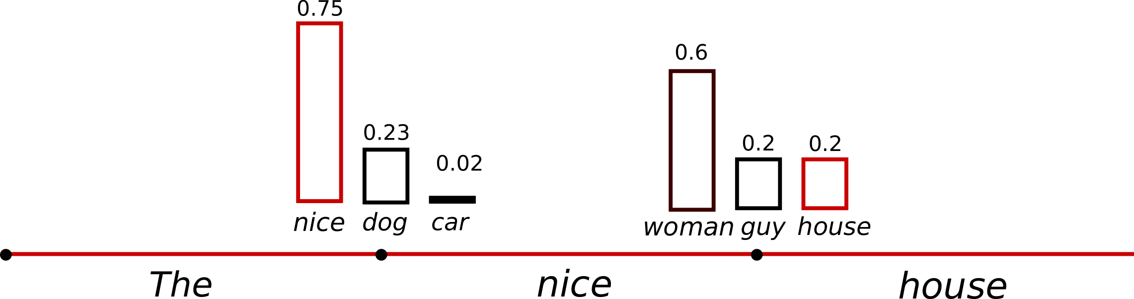
The conditional next word distribution of step $t=1t=1$ becomes much sharper leaving almost no chance for word $(\text{"car"})(\backslash text\{"car"\})$ to be selected.

Let's see how we can cool down the distribution in the library by setting temperature=0.6:

# set seed to reproduce results. Feel free to change the seed though to get different results
set_seed(42)

# use temperature to decrease the sensitivity to low probability candidates
sample_output = model.generate(
    **model_inputs,
    max_new_tokens=40,
    do_sample=True,
    top_k=0,
    temperature=0.6,
)

print("Output:\n" + 100 * '-')
print(tokenizer.decode(sample_output[0], skip_special_tokens=True))

Output:
----------------------------------------------------------------------------------------------------
I enjoy walking with my cute dog, but I don't like to chew on it. I like to eat it and not chew on it. I like to be able to walk with my dog."

So how did you decide

OK. There are less weird n-grams and the output is a bit more coherent now! While applying temperature can make a distribution less random, in its limit, when setting temperature $\to 0\backslash to\; 0$, temperature scaled sampling becomes equal to greedy decoding and will suffer from the same problems as before.

Top-K Sampling

Fan et. al (2018) introduced a simple, but very powerful sampling scheme, called Top-K sampling. In Top-K sampling, the K most likely next words are filtered and the probability mass is redistributed among only those K next words. GPT2 adopted this sampling scheme, which was one of the reasons for its success in story generation.

We extend the range of words used for both sampling steps in the example above from 3 words to 10 words to better illustrate Top-K sampling.

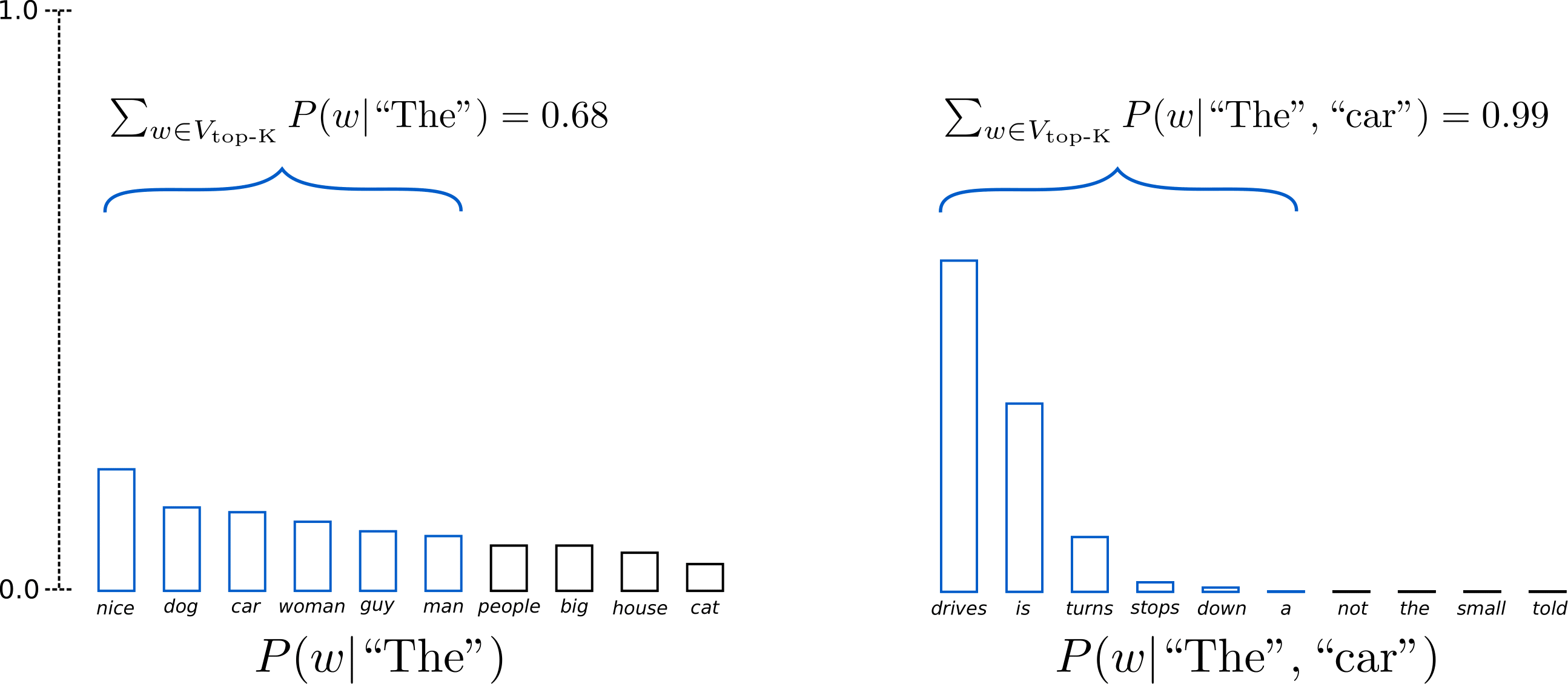
Having set $K=6K\; =\; 6$, in both sampling steps we limit our sampling pool to 6 words. While the 6 most likely words, defined as $V_{\text{top-K}}V\_\{\backslash text\{top-K\}\}$ encompass only ca. two-thirds of the whole probability mass in the first step, it includes almost all of the probability mass in the second step. Nevertheless, we see that it successfully eliminates the rather weird candidates $(\text{“not"},\text{“the"},\text{“small"},\text{“told"})(\backslash text\{``not"\},\; \backslash text\{``the"\},\; \backslash text\{``small"\},\; \backslash text\{``told"\})$ in the second sampling step.

Let's see how Top-K can be used in the library by setting top_k=50:

# set seed to reproduce results. Feel free to change the seed though to get different results
set_seed(42)

# set top_k to 50
sample_output = model.generate(
    **model_inputs,
    max_new_tokens=40,
    do_sample=True,
    top_k=50
)

print("Output:\n" + 100 * '-')
print(tokenizer.decode(sample_output[0], skip_special_tokens=True))

Output:
----------------------------------------------------------------------------------------------------
I enjoy walking with my cute dog for the rest of the day, but this time it was hard for me to figure out what to do with it. (One reason I asked this for a few months back is that I had a

Not bad at all! The text is arguably the most human-sounding text so far. One concern though with Top-K sampling is that it does not dynamically adapt the number of words that are filtered from the next word probability distribution $P(w\mathrm{\mid }{w}_{1:t-1})P(w|w\_\{1:t-1\})$. This can be problematic as some words might be sampled from a very sharp distribution (distribution on the right in the graph above), whereas others from a much more flat distribution (distribution on the left in the graph above).

In step $t=1t=1$, Top-K eliminates the possibility to sample $(\text{"people"},\text{"big"},\text{"house"},\text{"cat"})(\backslash text\{"people"\},\; \backslash text\{"big"\},\; \backslash text\{"house"\},\; \backslash text\{"cat"\})$, which seem like reasonable candidates. On the other hand, in step $t=2t=2$ the method includes the arguably ill-fitted words $(\text{"down"},\text{"a"})(\backslash text\{"down"\},\; \backslash text\{"a"\})$ in the sample pool of words. Thus, limiting the sample pool to a fixed size K could endanger the model to produce gibberish for sharp distributions and limit the model's creativity for flat distribution. This intuition led Ari Holtzman et al. (2019) to create Top-p- or nucleus-sampling.

Top-p (nucleus) sampling

Instead of sampling only from the most likely K words, in Top-p sampling chooses from the smallest possible set of words whose cumulative probability exceeds the probability p. The probability mass is then redistributed among this set of words. This way, the size of the set of words (a.k.a the number of words in the set) can dynamically increase and decrease according to the next word's probability distribution. Ok, that was very wordy, let's visualize.

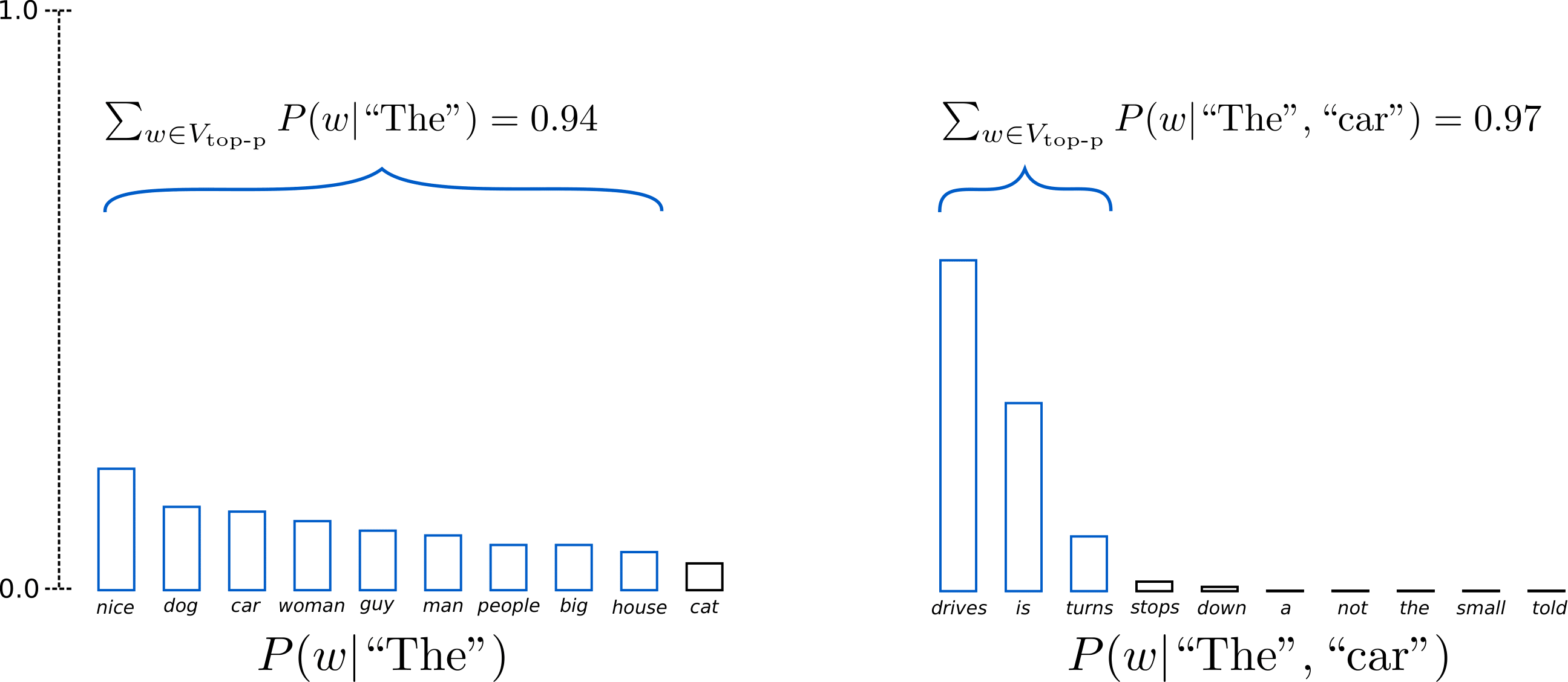
Having set $p=0.92p=0.92$, Top-p sampling picks the minimum number of words to exceed together $p=92\mathrm{\%}p=92\backslash \%$ of the probability mass, defined as $V_{\text{top-p}}V\_\{\backslash text\{top-p\}\}$. In the first example, this included the 9 most likely words, whereas it only has to pick the top 3 words in the second example to exceed 92%. Quite simple actually! It can be seen that it keeps a wide range of words where the next word is arguably less predictable, e.g. $P(w\mathrm{\mid }\text{"The”})P(w\; |\; \backslash text\{"The\text{'}\text{'}\})$, and only a few words when the next word seems more predictable, e.g. $P(w\mathrm{\mid }\text{"The"},\text{"car"})P(w\; |\; \backslash text\{"The"\},\; \backslash text\{"car"\})$.

Alright, time to check it out in transformers! We activate Top-p sampling by setting 0 < top_p < 1:

# set seed to reproduce results. Feel free to change the seed though to get different results
set_seed(42)

# set top_k to 50
sample_output = model.generate(
    **model_inputs,
    max_new_tokens=40,
    do_sample=True,
    top_p=0.92,
    top_k=0
)

print("Output:\n" + 100 * '-')
print(tokenizer.decode(sample_output[0], skip_special_tokens=True))

Output:
----------------------------------------------------------------------------------------------------
I enjoy walking with my cute dog for the rest of the day, but this had me staying in an unusual room and not going on nights out with friends (which will always be my yearning for such a spacious screen on my desk

Great, that sounds like it could have been written by a human. Well, maybe not quite yet.

While in theory, Top-p seems more elegant than Top-K, both methods work well in practice. Top-p can also be used in combination with Top-K, which can avoid very low ranked words while allowing for some dynamic selection.

Finally, to get multiple independently sampled outputs, we can again set the parameter num_return_sequences > 1:

# set seed to reproduce results. Feel free to change the seed though to get different results
set_seed(42)

# set top_k = 50 and set top_p = 0.95 and num_return_sequences = 3
sample_outputs = model.generate(
    **model_inputs,
    max_new_tokens=40,
    do_sample=True,
    top_k=50,
    top_p=0.95,
    num_return_sequences=3,
)

print("Output:\n" + 100 * '-')
for i, sample_output in enumerate(sample_outputs):
  print("{}: {}".format(i, tokenizer.decode(sample_output, skip_special_tokens=True)))

Output:
----------------------------------------------------------------------------------------------------
0: I enjoy walking with my cute dog for the rest of the day, but this time it was hard for me to figure out what to do with it. When I finally looked at this for a few moments, I immediately thought, "
1: I enjoy walking with my cute dog. The only time I felt like walking was when I was working, so it was awesome for me. I didn't want to walk for days. I am really curious how she can walk with me
2: I enjoy walking with my cute dog (Chama-I-I-I-I-I), and I really enjoy running. I play in a little game I play with my brother in which I take pictures of our houses.

Cool, now you should have all the tools to let your model write your stories with transformers!

Conclusion

As ad-hoc decoding methods, top-p and top-K sampling seem to produce more fluent text than traditional greedy - and beam search on open-ended language generation. There is evidence that the apparent flaws of greedy and beam search - mainly generating repetitive word sequences - are caused by the model (especially the way the model is trained), rather than the decoding method, cf. Welleck et al. (2019). Also, as demonstrated in Welleck et al. (2020), it looks as top-K and top-p sampling also suffer from generating repetitive word sequences.

In Welleck et al. (2019), the authors show that according to human evaluations, beam search can generate more fluent text than Top-p sampling, when adapting the model's training objective.

Open-ended language generation is a rapidly evolving field of research and as it is often the case there is no one-size-fits-all method here, so one has to see what works best in one's specific use case.

Fortunately, you can try out all the different decoding methods in transfomers 🤗 -- you can have an overview of the available methods here.

Thanks to everybody, who has contributed to the blog post: Alexander Rush, Julien Chaumand, Thomas Wolf, Victor Sanh, Sam Shleifer, Clément Delangue, Yacine Jernite, Oliver Åstrand and John de Wasseige.

Appendix

generate has evolved into a highly composable method, with flags to manipulate the resulting text in many directions that were not covered in this blog post. Here are a few helpful pages to guide you:

• How to parameterize generate

• How to stream the output

• Full list of decoding options

• generate API reference

• LLM score leaderboard

If you find that navigating our docs is challenging and you can't easily find what you're looking for, drop us a message in this GitHub issue. Your feedback is critical to set our future direction! 🤗