Traditional clickstream product analytics (like button clicks and page views) is one of the most important datasets for anyone trying to build a successful product. Backend observability data – metrics, logs, traces – are operational, but equally essential.

In the age of AI, though, we have a different kind of data that mashes aspects of both together. I'm talking about the LLM traces and generations your AI agent or agentic workflows produce as they get stuff done.

This data is crucial for seeing whether your agent is actually doing its job. It's also rich with insights about how your users are using AI features, what they're trying to do, and even how they feel about the whole interaction.

Think about all your interactions with an AI in the last week and all the subtle (or not so subtle) emotional signals embedded in them. By analyzing these signals in aggregate, AI product teams can discover usage patterns, outlier behaviors, and problem areas.

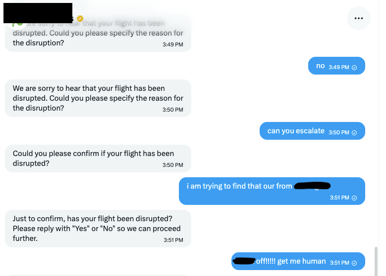
One of my recent interactions trying to chat with my airline about tickets.

Usually, analysis of these signals would take a set of complex queries and calculations, but since we have all this data in PostHog and we deal with this sort of complexity all the time, we built it for you.

It's aptly named "Clustering." We probably should have called it "Agentic AI-driven magic AI unicorn insights agentic" but engineers aren't the best at naming AI things.

Here's how the whole pipeline works under the hood, with links to the code if you want to dig deeper. If you just want to see it in action, skip to the demo.

Here's the overall flow from raw traces to clustered insights:

1. Ingest - Traces and generations land as PostHog events
2. Text representation - Convert each trace to a readable text format
3. Sample - Hourly sampling of N traces/generations
4. Summarize - LLM-powered structured summarization
5. Embed - Generate embedding vectors from summaries
6. Cluster - UMAP dimensionality reduction + HDBSCAN clustering
7. Label - An AI agent names and describes each cluster
8. Display - Clusters tab with scatter plot and distribution chart

Design considerations

Before diving into the steps, here are the main considerations we kept coming back to and the choices we made for each:

• Huge traces - Some traces are enormous and can't just be thrown at an LLM. Our answer: the uniform downsampling described below in step 1. We iteratively drop lines while preserving the overall structure, so even massive traces fit within context limits, although this is at the cost of some accuracy/quality.
• Keeping costs sane - Running LLM summarization on every single trace would cost a lot. So we sample a small random subset each hour, use GPT-4.1 nano for summarization (fast and cheap), and are planning to move to the OpenAI Batch API to optimize further, as well as some BYOK approaches for "on demand" steering and triggering of the whole pipeline.
• One-size-fits-all vs. custom summaries - It's hard to have a single general summary schema that works perfectly for every type of trace we might see. Ideally, users could steer or bring their own prompts and structured outputs. For now, we started with a general-purpose prompt and summary schema that works well across most use cases, but enabling user-defined summarization is a potential future improvement.
• No existing embeddings to lean on - PostHog doesn't already have a RAG system or embeddings index over all AI Observability events. Rather than building that infrastructure first, we took a shortcut: convert traces to text, summarize them with an LLM, then embed the summaries. This gives us high-quality, semantically rich vectors without needing a full RAG pipeline - and the summaries are useful on their own as a feature.
• Zero-config by default, customizable when you need it - The Temporal workflows just run in the background. As you send traces to AI Observability, clustering will just work once there's enough data to sample from. No setup needed — but if you want more control, you can now create clustering jobs to steer what gets clustered (more on this below).
• User steering - We recently shipped clustering jobs, which let you define up to five independent clustering configurations per project. Each job can target a specific analysis level (traces or generations) and apply event filters to scope which data gets included — for example, you could create a job that only clusters traces from a specific model or a particular user segment. Jobs run automatically during the next scheduled cycle.

Step 1: From JSON blobs to readable text

Traces are ingested into AI Observability as normal PostHog events. They have their own loose schema around special $ai_* properties – covering everything from generations and spans to sessions – but also the flexibility of general PostHog events, which means they generally work with any other PostHog feature out of the box.

This gives us a blob of JSON with some expected $ai_ properties, and even within each property, the structure and format can vary wildly depending on the LLM provider, framework, or how users have instrumented their own agents.

So we need to figure out how to get from this bag of JSON to something a clustering algorithm can work with – we need numbers. And whenever you need numbers with LLMs, it often means you need embeddings. Our task is to figure out what embeddings to generate that will be useful downstream.

We can't just throw some massive JSON blob at an LLM and expect it to produce a great summary. It might be okay, but we can do better by putting ourselves in the shoes of our LLM: if I can create a general text representation where I myself can easily "read" a trace, then that'll also be a great input for summarization. We be context engineering like the AI hipsters we aspire to be.

So we built a process that renders each trace (or any event in it) as a clean, simple text representation – essentially an ASCII tree with line numbering. The idea here is just some simple text so you can "read" the trace, you know, as a human.

Here's what it looks like in the PostHog UI:

You can see the full text representation for this trace in this gist — it's a real example from one of my side projects (a daily factoids chatbot that got into a surprisingly deep conversation about mantis shrimp vision and digital signal processing). Point being, if its easier for me as a human to grok what's going on, the LLM should be able to do a decent job of summarizing it with less risk of getting side tracked by all the other gnarly metadata and structure in the raw JSON.

The line numbering (L001:, L002:) is important – it gives the downstream summarization LLM a way to reference specific parts of the trace, which makes the structured output much more useful.

You can see how this is generated in trace_formatter.py.

Handling huge traces

Some traces are just too big. We use uniform downsampling to shrink them – picking every Nth line from the body while preserving the header. The sampler notes what percentage of lines were kept, and the gaps in line numbers tell the LLM that content was omitted. Using the mantis shrimp trace from the gist, here's a snippet of what a downsampled version might look like:

Notice the [SAMPLED VIEW: ~40% of 136 lines shown] header and the jumps in line numbers (e.g., L051 → L059, L079 → L101). The LLM can still follow the conversation flow – the structure and key turns are preserved, just with less detail in between. This works well in practice because the same context often gets passed back and forth within each step of a trace.

See how downsampling works in message_formatter.py.

Now that we have a readable text representation, we can summarize it. We sample N traces per hour (cost management – we're not summarizing everything) and send each text representation to an LLM for structured summarization.

The key word there is structured. Rather than asking for a free-text summary, we ask for a specific schema:

See the full summarization schema in schema.py

We use GPT-4.1 nano for this – it's fast, cheap, and the structured output mode means we get reliable, parseable results every time. The line references back to the text representation are particularly useful: they let the summary stay grounded in the actual trace data rather than hallucinating. You can read the actual prompts we use in system_detailed.djt and user.djt. If you have sensitive data in your traces, we made sure clustering works with privacy mode which controls what gets sent.

These summaries appear as $ai_trace_summary and $ai_generation_summary events in your project every hour. They also power the on-demand trace summarization feature you can use to quickly understand any individual trace or generation without reading through the full conversation.

Ideally we would enable users the ability to steer and customize this part of the flow – maybe you want a different summary schema, or you want to add specific questions for the LLM to answer in the summary. We're considering this for the future, but for now we started with a general-purpose schema that works decently across most use cases.

Why structured output matters

Structured output is better than a raw summary for one critical reason: downstream embedding quality. When we embed a title + flow diagram + specific bullets with line references, we get a much higher signal representation than embedding a wall of free text. The LLM has already done the work of extracting what matters.

Why not RAG? We considered building a full RAG system – chunking traces, building indices, retrieving at query time. But the complexity of doing that well at PostHog's scale (billions of events across thousands of teams) made us reach for a simpler approach first. Summarization-first means each trace becomes a small, self-contained artifact that's easy to embed and cluster. We may still build RAG for features like natural language search, but for clustering, this works well.

Once we have summaries, we format them back into plain text – title, flow diagram, bullets, and notes concatenated together, with line numbers stripped to reduce noise – and embed them using OpenAI's text-embedding-3-large model, giving us a 3,072-dimensional vector for each summary.

Why embed the enriched summary instead of the raw trace? Because the summary lives in a higher-level semantic space. Raw traces contain a lot of noise – token counts, model versions, repeated system prompts. The summary captures the intent and flow, which is exactly what we want our clusters to be organized around.

So now, for each trace or generation, we have 3,072 numbers. Time for the fun part.

This is where we lean on more "old school" traditional ML techniques. There are still several areas where LLMs haven't eaten the world: recommender engines, clustering, time series modeling, tabular model building, and getting well-calibrated numbers for regression problems. For all of these, you're still better off equipping your agent with the tools to formulate and run traditional algorithms on the data, rather than asking it to do the calculations directly.

Dimensionality reduction

We can't just cluster the raw 3,072-dimensional vectors – the curse of dimensionality would make distances meaningless. So we first need to reduce dimensions while preserving the important structure.

We run UMAP, an algorithm for reducing high-dimensional data while preserving local structure, twice with different goals:

• 3072 → 100 dimensions for clustering: min_dist=0.0 packs similar points tightly together, which is what HDBSCAN wants.
• 3072 → 2 dimensions for visualization: min_dist=0.1 keeps some visual separation so the scatter plot is readable.

HDBSCAN

UMAP's job was dimensionality reduction — compressing 3,072 dimensions into something workable while preserving structure. HDBSCAN is the algorithm that actually finds the clusters by scanning the reduced space for dense regions of similar points and grouping them together. For the actual clustering, we use HDBSCAN on the 100-D reduced embeddings:

See the full UMAP + HDBSCAN pipeline in clustering.py

HDBSCAN has some nice properties for our use case:

• No need to pick k (number of clusters) in advance - it figures this out automatically based on density.
• Noise cluster - items that don't fit any cluster get assigned to cluster -1. These "outliers" can be interesting edge cases you might want to explore.
• cluster_selection_method="eom" (Excess of Mass) tends to produce more granular, interpretable clusters compared to the "leaf" method.

After this step, every trace or generation has an integer cluster ID. But an integer doesn't tell you much – we need to make these meaningful.

Now we have clusters with integer IDs. Cluster 0 has 47 traces, cluster 1 has 23, cluster -1 (noise) has 8. Not exactly actionable.

This is where we bring AI back in – specifically, a LangGraph ReAct agent powered by GPT-5.2. Its job is to explore the clusters and come up with meaningful labels and descriptions.

You can read the agent's system prompt in prompts.py.

The agent has access to 8 tools:

The agent starts with a bulk-labeling phase: it calls get_all_clusters_with_sample_titles for an overview, then uses bulk_set_labels to assign initial labels to every cluster. This guarantees coverage — if the agent hits a token limit or error later, no cluster is left unlabeled.

Then it moves to refinement. For clusters that seem ambiguous, it drills deeper with get_cluster_trace_titles and get_trace_details, then calls set_cluster_label to update individual labels. Finally, it calls finalize_labels to signal completion.

See the agent tools and prompts in labeling_agent/

All of this needs to run reliably across thousands of teams. We use Temporal workflows to orchestrate the pipeline.

A daily coordinator workflow discovers eligible teams (those with enough recent trace data), then spawns child workflows in batches – up to 4 concurrent workflows at a time to manage load. These workflows:

1. Fetch recent embeddings
2. Run clustering pipeline (UMAP + HDBSCAN)
3. Run labeling agent
4. Emit cluster events

See the orchestration workflow in coordinator.py

The output of each child workflow is a set of $ai_trace_clusters and $ai_generation_clusters events. These are standard PostHog events, which means the clusters tab in the UI is just querying events like everything else in PostHog.

Here's what you're seeing in the demo:

• Scatter plot - Each dot is a trace, positioned using the 2-D UMAP coordinates. Colors represent cluster assignments. You can immediately see which groups of traces are similar and how they relate spatially.
• Cluster distribution - A bar chart showing how many traces landed in each cluster, with the agent-generated labels. This gives you a quick sense of what your users are actually doing.
• Drill-down - Click into any cluster to see the individual traces, their summaries, and the full details. This is where you find the patterns - maybe 40% of your traces are "user asking for refund status" and you didn't even know.

The noise cluster (labeled "Outliers") often contains the most interesting one-off traces – edge cases, unusual workflows, or bugs that don't fit any pattern. Pair this with evaluations (our LLM-as-a-judge feature) to automatically score the quality of generations within each cluster.

Since launching this pipeline, we've added clustering jobs — a way to create independent clustering configurations so you can steer what gets analyzed. Instead of one big clustering run across all your data, you can define up to five jobs per project, each with its own analysis level (traces or generations) and event filters.

For example, you might create separate jobs for:

• Traces from your production GPT-4o agent
• Generations from your RAG pipeline
• Only traces where a specific custom property matches (e.g., $ai_model = "claude-sonnet-4-20250514")

Each job runs automatically during the next scheduled cycle, and the run selector on the Clusters page shows which job produced each run. See the clustering jobs docs for the full setup guide.

If you're already using AI Observability in PostHog, clustering runs automatically – no configuration needed. Want more control? Set up clustering jobs to define exactly what gets clustered. If you're not using AI Observability yet, you can get started in minutes with SDKs for OpenAI, Anthropic, LangChain, Vercel AI, and many more.

Try clusters in PostHog

• Clusters documentation - Setup guide and feature overview
• Custom properties - Attach your own metadata to traces for richer clustering
• Privacy mode - Control what trace data gets sent to PostHog
• Feedback - Leave feedback directly on the clusters docs page, email us at team-llm-analytics@posthog.com, or start a thread in the community